Private doesn’t mean lonely. Signal’s mission is to help you connect with people
in a secure way. This means that you need to know which of your contacts are
also on Signal. This is called “contact discovery” and it’s an essential part of
any messaging app.
Most other communications apps enable contact discovery by maintaining their own
internal social graph or by uploading and storing your full address book on
their servers. But Signal enables you to find and connect with people in a
privacy-preserving way. In short, we let you see which of your friends use
Signal, but we don’t want to know who your friends are. Letting you know which
of your contacts are using Signal while preserving the privacy of your social
map requires some complex engineering choices on our end.
In this post, we’ll be diving into some new ways that improve our ability to
handle contacts in a private way. That’s right folks. We’re getting technical.
We’re talking enclaves and memory access patterns. [If you’ve never heard of an
enclave before, don’t worry. We’ll explain it soon.]
Our new method is faster and more efficient. It lays the groundwork for the
introduction of usernames and phone number privacy which will offer new privacy
controls around your phone number’s visibility on Signal.
On September 12 I’ll be stepping into the role of Signal’s President, a new
position created in collaboration with Signal’s leadership. I am thrilled, and I
can’t think of a more meaningful use of my time, or a greater honor. I’ve been a
friend, admirer, and champion of Signal since it was RedPhone and TextSecure,
and in 2020 I joined Signal’s Board of Directors, helping inform high-level
strategy and direction. So in many ways this is a happy step on a long
continuum, not a dramatic change.
Signal is more important now than ever, and I expect this to stay true well into
the future. As President I will dedicate myself to helping Signal build a long
taproot so it can grow and thrive in dynamic climates. In this role I will be
working with Signal’s CEO and leadership, with a particular focus on guiding
Signal’s strategy, ensuring our financial sustainability, sharpening and
broadening Signal’s public communications, and whatever else is needed to
strengthen the app and the org.
Signal is currently blocked in Iran. To help people in the country access
Signal, we are republishing and revising a post that we
originally posted in February, 2021 during a very similar situation in Iran.
If you are willing and able, please follow the instructions below to set up a
proxy server that will enable people in Iran to connect to Signal. We are
grateful to the community who pitches in to help each other during these
moments.
If you are currently running a proxy, you will need to make some updates to
ensure it continues to function. Update instructions are
here.
For many years, the Signal app on Android has supported sending and receiving plaintext SMS and MMS messages in addition to Signal messages. SMS and MMS are standardized communication protocols that allow mobile devices to send and transmit messages, and most people picking up their phone to text or share memes don’t really think about them.
To give some context, when we started supporting SMS, Signal didn’t exist yet. Our Android app was called TextSecure and the Signal encryption protocol was called Axolotl. Almost a decade has passed since then, and a lot has changed.
The tech industry–its products, conceptual frameworks, linguistic conventions, and cultural norms–is largely centered in the US (and, increasingly, China. But we’re focused here on the US, where Signal is based). This is not because the US has better programmers or more visionary entrepreneurs, but due primarily to historical material conditions. For example, early investments in networked computation from the US military, which happened around the same time that the US was becoming a global superpower, which was followed by the privatization and then commercialization of networked computation, then the dot com boom, etc. etc., and here we are.
Signal exists to provide people everywhere with a tool for real private communication. That’s our only goal, and we take it very seriously. We’re structured as a nonprofit to ensure that market forces can never put profit or expediency over the safety of those who rely on us. Our work also resonates beyond the Signal app. The Signal Protocol has become the foundation for end-to-end encryption technology that is used and trusted by many private messaging services to protect billions of messages every day.
We recognize that privacy is a human right and that free expression and the ability to dissent are fundamental to a safe and vibrant society. But the current state of the Online Safety Bill in the UK puts the future of privacy and expression in grave jeopardy.
The Signal Protocol is a set of cryptographic specifications that provides
end-to-end encryption for private communications exchanged daily by billions of
people around the world. After its publication in 2013, the Signal Protocol was
adopted not only by Signal but well beyond. Technical information on the Signal
Protocol can be found in the specifications section of our docs site.
Today we are happy to announce the first step in advancing quantum resistance
for the Signal Protocol: an upgrade to the X3DH specification which we
are calling PQXDH. With this upgrade, we are adding a layer of
protection against the threat of a quantum computer being built in the future
that is powerful enough to break current encryption standards.
This post is written to introduce this work to non-experts, and will review what
quantum computing is and the challenges it presents for current cryptographic
algorithms, before providing a high level overview of how we are adapting our
specifications to answer these challenges. If you would like to skip this
summary and explore our PQXDH specification in depth, you can read our technical
whitepaper here.
You should be able to communicate without worrying that every gossip tidbit, meme, or joke you share and who you share it with will get churned up into fodder for targeted ads or used to train an AI model. You also shouldn’t have to strip your communications down to the barest and most utilitarian version of relaying information.
This is why Signal is dedicated to providing a truly private messaging app, and why we work to constantly make the experience better for everyone who uses it.
We want you to know about the improvements we’re making in Signal, even the smaller ones that simply make the app nicer to use. So, starting here we’re publishing a periodic New Features Roll Call, reviewing multiple new features and quality of life improvements in one place.
Signal is the world’s most widely used truly private messaging app, and our cryptographic technologies provide extra layers of privacy beyond the Signal app itself. Since launching in 2013, the Signal Protocol—our end-to-end encryption technology—has become the de facto standard for private communication, protecting the contents of billions of conversations in WhatsApp, Google Messages, and many others. Signal also continues to invest in research and development in the pursuit of extending communications privacy. This commitment underlies our recent work to add a layer of quantum resistance to the Signal Protocol, and our previous work on metadata protection technologies that help keep personal details like your contact list, group membership, profile name, and other intimate information secure. This singular focus on preserving the ability to communicate privately is one reason that we work in the open, documenting our thinking and making our code open source and open to scrutiny—so you don’t have to take our word for it.
In just the past few years, large machine learning models have made incredible strides. Today’s models are not only remarkably capable but also achieve impressive results across a range of applications, from software engineering and scientific research to content creation and data analysis. With the arrival of models like Kimi-K2.5 and GLM-5, the pace of progress shows no sign of slowing down. (Kimi-K2.5 has an impressive 1 trillion parameters, nearly twice as many as the DeepSeek V3 model family that was released just last year.) And as these models continue to grow in size and capability, so does the demand for memory, computing power, and energy.
One of the most effective ways teams are addressing these constraints is through low-bit inference, a set of techniques widely adopted across the industry that make AI models faster and cheaper to run by reducing how much memory and compute they need when serving real user requests. At Dropbox, products like Dropbox Dash rely on various models to deliver fast, reliable, and cost-effective AI-powered search and understanding across vast amounts of user content. Making this possible requires careful attention to model efficiency, hardware utilization, and latency constraints. And making this technology accessible to individuals and businesses means tackling new challenges around efficiency and resource use.
In this article, we’ll dive into the current landscape of low-bit compute for efficient inference. We’ll cover the different types of quantization, why and when they’re needed, and the key optimization challenges required to deploy advanced AI models in production.
Dropbox Dash: AI that understands your work
Dash knows your context, your team, and your work, so your team can stay organized, easily find and share knowledge, and keep projects secure, all from one place. And soon, Dash is coming to Dropbox.
At Dropbox, almost all the models used in-house are attention-based architectures used for tasks like understanding text, images, videos, and audio—core capabilities behind Dash’s ability to search, summarize, and reason over large collections of user content. As these models grow in size and complexity, efficiently serving them in production becomes a central challenge for delivering responsive user experiences. In attention-based models, most of the compute comes from repeated matrix multiplications in two main parts of the model:
The first is the linear layers, which compute embeddings throughout the model. These include:
The layers used within attention blocks, the components that determine how different parts of the input relate to one another
MLP layers, which further process and refine those representations
The model’s final output stage, where those representations are converted into a concrete result, such as a prediction or response.
The second is the attention mechanism itself, where the model evaluates relationships across the input to determine which information is most relevant, a step that significantly increases compute cost with longer context sizes.
On GPUs, these matrix multiplications are handled by specialized hardware. NVIDIA GPUs use Tensor Cores, while AMD GPUs use Matrix Cores. These dedicated processors are accessed through matrix multiply-accumulate (MMA) instructions and are designed specifically to accelerate matrix operations—the heavy-duty math that underpins large-scale linear algebra in neural networks—delivering substantial performance gains compared to executing the same work on general-purpose CUDA Cores.
One notable property of these cores is their scaling behavior. As numerical precision is reduced, these cores can perform more matrix operations per second, typically resulting in higher FLOPS (floating point operations per second, or how much math the hardware can do in a given time). In practice, halving the precision often allows these cores to roughly double throughput. This scaling behavior plays a key role in improving both performance and efficiency when running large-scale AI workloads.
Fig. 1: Tensor Core dense matrix multiplication performance (FLOPs) across different NVIDIA RTX 6000 variants and data precisions
Lowering numerical precision is accomplished through quantization, a technique that reduces the number of bits used to represent numerical values. By quantizing tensors, for example, from 16-bit to 8-bit or 4-bit, the memory footprint is reduced because each element requires fewer bits. This is typically done by rescaling the data to fit within a smaller representable range. For instance, 8-bit quantization maps values to 256 bins, restricting each tensor element to one of these discrete levels while approximating the original floating-point values. Quantization to lower than 8 bits typically requires an additional process called bitpacking, where multiple low-bit elements are combined into a native data type such as uint8 or int32, since 4-bit formats are not natively supported.
Lowering precision not only improves speed and memory usage, but also improves energy efficiency, since lower-bit data requires less power for both memory transfer and computation. For instance, with FP4 support, Blackwell offers significant energy savings compared to the H100.
There have also been attempts to explore lower bits such as binary and ternary weights (restricting weights to two or three discrete levels), which would offer even more theoretical energy efficiency. However, this form of quantization isn’t well suited for modern GPUs because it can’t fully leverage Tensor/Matrix Cores. Although there have been experimental efforts to explore custom hardware or specialized accelerators tailored to such schemes, this approach hasn’t yet seen broad industry adoption as a result of limited ecosystem support and model quality concerns. In short, while lower precision can dramatically improve efficiency, real-world gains depend on how well those formats are supported by existing hardware and software ecosystems.
In the following section, we examine different quantization configurations and highlight their key trade-offs when deployed on modern GPUs.
Understanding quantization formats
Quantization is not a single technique, but a family of approaches that differ in how numerical values are represented, scaled, and executed on hardware. These design choices directly affect model accuracy, performance, and how efficiently modern GPUs can accelerate inference. As a result, quantization formats are closely tied to the capabilities and constraints of the underlying hardware.
In practice, these differences matter because Dropbox runs a diverse set of AI workloads—such as multimedia understanding—across multiple generations of hardware, each with distinct performance characteristics. Some workloads are highly latency sensitive, prioritizing fast per-request execution, while others are throughput oriented and optimized for processing large volumes of data efficiently. Quantization formats influence how well a model can adapt to these constraints, determining whether computation is bound by software overhead, memory bandwidth, or specialized hardware units like Tensor Cores. Framing quantization through this lens helps clarify why different formats unlock different tradeoffs across our stack, and why no single approach is optimal for every workload we deploy.
With the introduction of the MXFP microscaling format, which standardizes low-bit data types with native hardware support, quantization methods for large language models can be broadly grouped into two categories: pre-MXFP formats, which rely on explicit dequantization and software-managed scaling, and MXFP formats, which move these operations directly into Tensor Core hardware. The sections below walk through both approaches, highlighting how they differ in practice and why those differences matter for real-world inference workloads.
Pre-MXFP formats
Prior to the introduction of MXFP, quantization primarily relied on integer data types for sub-byte formats. Common configurations included A16W4 (16-bit activations, 4-bit weights) for weight quantization, and either integer or floating-point formats for activations, such as A8W8 (8-bit activations, 8-bit weights). In contrast, sub-byte weight quantization generally requires calibration or more advanced algorithms to maintain model quality. For example, A16W4 relies on techniques such as AWQ or HQQ—quantization methods designed to preserve model quality at low bit widths—while lower-bit formats like A16W3, A16W2, and BitNet require increasingly sophisticated training quantization methods to achieve acceptable accuracy.
When activations and weights use different data types, the typical approach is to explicitly dequantize the lower-bit tensors to match the higher-precision format before performing the matrix multiplication (MMA) operation. This strategy can improve performance in memory-bound scenarios, where reducing data movement is the primary concern. However, in compute-bound workloads, the additional dequantization step can offset these gains and even slow execution due to the extra arithmetic involved.
This trade-off is especially visible in weight-only quantization, which reduces data transfer but does not accelerate the extra computation required to run matrix multiplications. The choice between activation quantization (such as A8W8) and weight-only quantization (such as A16W4) ultimately depends on the characteristics of the inference workload. Weight-only quantization often performs better in local deployments with smaller batch sizes and reasoning-heavy tasks, where memory bandwidth is a limiting factor. In contrast, activation quantization tends to be more effective for large-context prefills and high-throughput serving scenarios, where compute becomes the dominant bottleneck.
Fig. 2: A8W8 vs. A16W4 decoding performance across various batch sizes. A8W8 tends to outperform A16W4 in more compute-bound scenarios. A16W4 tends to perform worse than 16-bit matrix multiplication due to the additional cost of explicit dequantization
Popular methods such as AWQ and HQQ rely on linear quantization with grouping, a design that balances efficiency with accuracy. In symmetric linear quantization, dequantization is expressed as a simple scaling operation. A more flexible variant, asymmetric linear quantization, introduces an additional offset, allowing dequantization to be implemented as a fused multiply-add operation that maps efficiently to modern GPU hardware.
Grouping further improves accuracy by assigning shared parameters to small blocks of tensor elements rather than individual values. These groups typically consist of contiguous elements of size 32, 64, or 128. While simple, this approach substantially reduces quantization error at low-bit widths and has become a core component of most practical low-bit quantization schemes.
Fig. 3: Linear quantization overview where a matrix W is decomposed into Wq (low-bit tensor) and additional floating-point scales (s) and zero-points (z)
On the activation side, two 8-bit approaches are commonly used: channel-wise quantization and per-block quantization. Channel-wise quantization is straightforward and efficient, making it well suited for on-the-fly inference. The required rescaling can be applied directly after matrix multiplication, allowing for a highly efficient implementation on modern GPUs.
Per-block quantization, popularized by systems such as JetFire and DeepSeek V3, takes a more fine-grained approach. By dividing tensors into small tiles and assigning an independent scale to each block, this method limits the impact of outliers and reduces quantization error. It is particularly effective in quantization-aware training, where preserving pre-training accuracy is critical, while still delivering practical Tensor Core speedups.
Beyond linear quantization, several non-linear approaches, including QuiP# and GPTVQ, have explored alternative representations to push precision even lower. While these methods can achieve higher accuracy at very low-bit widths, they face practical challenges. Linear 4-bit quantization already delivers strong accuracy and can often be applied on the fly using techniques such as HQQ, avoiding expensive offline quantization passes. In addition, deploying non-linear formats efficiently requires custom fused kernels and deep integration into inference frameworks. Even then, low-bit weights must still be converted into a form compatible with Tensor Cores, making linear quantization both simpler and more practical on current GPU architectures.
Quantization techniques are also well-suited for optimizing the attention module. Methods such as Flash Attention 3 and Sage Attention use 8-bit quantization to accelerate attention-related matrix multiplications, improving throughput and memory efficiency with minimal impact on model accuracy.
MXFP formats
The MXFP microscaling format introduces a new standard for low-bit data types that fundamentally changes how quantized models run on modern GPUs. Unlike earlier formats, MXFP provides native hardware support for quantization, allowing Tensor Cores to operate directly on quantized activations, weights, and their associated scaling factors in a single fused operation. In contrast, pre-MXFP approaches required explicit dequantization steps before or after matrix-multiply-accumulate (MMA) operations, adding overhead and limiting achievable performance.
MXFP quantizes both activations and weights using a micro-scaling approach, similar in spirit to methods like AWQ and HQQ discussed earlier, but implemented directly in hardware. It uses symmetric quantization with a fixed block size of 32 and applies shared scaling factors stored in the E8M0 format. MXFP also supports mixed-precision MMA operations on some hardware, such as MXFP8 × MXFP4, giving practitioners flexibility to balance performance and accuracy. For example, activations can use MXFP8, MXFP6, or MXFP4 while the weights can remain in MXFP4. A breakdown of the MX types is demonstrated in the table below (source: Open Compute Project, OCP Microscaling Formats (MX) Specification, Version 1.0, Table 1).
Fig. 4: MX dtype breakdown
The E8M0 format for the scales represents positive powers of two in the range [2⁻¹²⁷, 2¹²⁷]. The scales are typically quantized as follows: scale = weight.amax(axis=1, keepdim=True) / max_val. As a result, scale values are effectively limited to values at or below 1, and extremely small magnitudes are rarely needed. In many cases, values as small as 2⁻¹⁵ are sufficient to capture near-zero weights. This observation suggests that scales could theoretically be represented with fewer bits than E8M0, although doing so would introduce additional complexity.
While E8M0 offers hardware-friendly implementation and flexibility, constraining scale values strictly to powers of two leads to a noticeable accuracy drop when using MXFP4. Fortunately, this loss can largely be mitigated through simple post-training adjustments, restoring most of the original model quality, as we demonstrated in our blog post.
To address remaining numerical limitations, NVIDIA introduced NVFP4 as an alternative to MXFP4. NVFP4 uses a smaller group size of 16 rather than 32 and employs E4M3 FP8 scaling factors, providing higher precision for scale representation. Because FP8 has a relatively large minimum representable value, a global per-tensor floating-point multiplier is applied to normalize the scaling range, achieving improved numerical stability.
Although MXFP4 and NVFP4 are standardized formats, their implementation depends on the GPU architecture. Different compute capabilities rely on different Tensor Core instructions. For example, sm_100 architectures use the tcgen05.mma instruction, while sm_120 architectures use mma.sync, both incorporating the block_scale modifier. As a result, kernels compiled for sm_100 are not portable to sm_120 due to these instruction-level differences. While most of the mainstream AI software stack remains focused on server-grade GPUs like the B200 and B300, there has been significant recent progress toward improving portability of low-bit workloads. Notably, Triton has introduced support for MXFP on sm_120 devices, enabling greater flexibility and cross-device compatibility for low-bit Triton kernels.
Looking forward
In this article, we explored several quantization techniques that are widely adopted across the industry to accelerate AI workloads. These approaches unlock substantial gains in efficiency and throughput, making it possible to deploy increasingly large and capable models within practical hardware, cost, and energy constraints.
At Dropbox, these considerations are central to how we build and operate products like Dash. Dash relies on large-scale models for experiences such as conversational AI, multimodal search, document understanding, and speech processing, all of which must meet strict latency, reliability, and cost requirements. To satisfy these constraints in production, we already employ a range of quantization strategies to optimize model deployment and fully utilize modern accelerators. The techniques discussed here reflect the kinds of trade-offs we evaluate when deciding how and where to run models across our infrastructure.
Despite the progress, important limitations remain. In real-world deployments, adoption of formats such as MXFP and NVFP is still evolving, and support for FP4 quantization remains incomplete across popular frameworks and model stacks. For example, many open-source runtimes don’t yet provide full support across different GPU architectures, and FP4 models are not yet widely available.
As hardware continues to evolve and the industry pushes toward lower-bit compute, these challenges will only become more pronounced. In our view, making low-bit inference viable for production systems like Dash will require tighter software design, more mature framework support, and new quantization techniques that preserve model quality at scale. We view this as an active area of exploration, one that will directly shape how we deliver fast, reliable, and efficient AI-powered experiences to Dropbox users in the years ahead.
~ ~ ~
If building innovative products, experiences, and infrastructure excites you, come build the future with us! Visit jobs.dropbox.com to see our open roles.
Signal’s mission and sole focus is private communication. For years, Signal has kept your messages private, your profile information (like your name and profile photo) private, your contacts private, and your groups private – among much else. Now we’re taking that one step further, by making your phone number on Signal more private.
When someone uses Dropbox Dash to search or ask a question, it follows a retrieval-augmented generation (RAG) pattern. This means our AI first retrieves relevant company information and then uses that information to generate responses. To produce those answers, it relies on enterprise search to retrieve company-specific context and then uses that context to ground the response. Rather than responding solely from general knowledge, Dash incorporates information that already exists within an organization.
When a user submits a query, Dash first interprets the underlying information need and determines how to retrieve relevant content. Search returns a set of candidate documents, and a large language model (LLM) analyzes the most relevant results to generate an answer. Because there are millions (and, in very large enterprises, billions) of documents in the enterprise search index, Dash can pass along only a small subset of the retrieved documents to the LLM. This makes the quality of search ranking—and the labeled relevancedata used to train it—critical to the quality of the final answer.
Search results in Dash are ordered by a relevance model that assigns a score to each document based on how well it matches the query. Like most modern ranking systems, this model is trained rather than hand-tuned. It learns from examples of queries paired with documents, annotated with human relevance judgments that define what high-quality search results look like. These judgments are labeled examples in which people evaluate how well a document answers a given query.
In this story, we explain how we train Dash's search ranking models with a mix of human and LLM-assisted labeling—starting with a small amount of internal, human-labeled data, and then amplifying those efforts with LLMs to produce relevance labels at scale.
Dropbox Dash: AI that understands your work
Dash knows your context, your team, and your work, so your team can stay organized, easily find and share knowledge, and keep projects secure, all from one place. And soon, Dash is coming to Dropbox.
Dash’s ranking model is trained using machine learning techniques such as XGBoost rather than manually tuned rules. It learns from labeled examples of query–document pairs, where each document is evaluated based on how well it satisfies a given query. Over time, the model adjusts how it weighs different signals to reduce ranking mistakes (for example, cases where less useful documents are placed ahead of more useful ones). This framing leads directly to a core challenge: generating enough high-quality relevance labels to train the model effectively.
Where relevance labels come from
Training a relevance model requires examples that show what “good” and “bad” search results look like. In practice, those relevance labels can be created in several ways. One approach infers relevance from user behavior, such as clicks or skipped results. Another relies on humans manually assigning relevance scores to query and document pairs. And a third approach uses LLMs to generate relevance judgments directly.
This story focuses on the latter two approaches: direct human labeling and LLM-based evaluation. Signals from user behavior can still be helpful, but on their own they tend to be incomplete, influenced by existing rankings, and unevenly distributed. In practice, they work best as a supplement to labeled data rather than a replacement for it.
For the purposes of this article, relevance is treated as a graded score on a 1–5 scale. A score of 5 means the result closely matches what the user is trying to find, while a score of 1 means it isn’t useful enough to show. Importantly, relevance isn’t a fixed property of a document; it depends on the specific query, the user’s context, and the moment the search is made.
Human labeling Historically, search engine providers relied on teams of human judges, typically third-party vendors, to label large datasets for model training. This approach had clear advantages. Human judges could systematically evaluate full result sets for each query, ensuring comprehensive and consistent relevance coverage in a way that user feedback—which is often sparse and biased—cannot.
However, the drawbacks are substantial. Human labeling is expensive and difficult to scale. Judges can be inconsistent and require ongoing training. In practice, it is also nearly impossible for humans to directly evaluate sensitive or proprietary customer data. Human evaluators also require training, which is made more difficult by the diversity of types of content that need to be rated (for example, comparing a Slack message to a Jira ticket or a Salesforce contact record can require very different contextual understanding and judgment).
LLM evaluation LLMs provide an alternative mechanism for producing relevance judgments at scale. Compared to human annotators, LLMs are significantly cheaper, more consistent, and capable of evaluating much larger candidate sets across languages. They can also analyze customer content within defined compliance boundaries.
At the same time, LLMs are not general intelligence systems. Their performance depends heavily on both the quality of the underlying model and the clarity and precision of the instructions provided. As a result, LLM-generated relevance judgments must be evaluated and calibrated carefully before they are used for training. In practice, using LLMs for relevance evaluation requires a structured process that combines automation with human oversight.
Combining LLM evaluation with human review
To scale relevance evaluation without sacrificing quality, Dash pairs automation with human judgment. Before deploying an LLM to generate relevance labels at scale, its performance is validated against a small, high-quality set of human-labeled examples. (Human review is conducted by Dropbox with limited, non-sensitive internal datasets; no customer data is reviewed by humans as part of this process.)
A small group of human evaluators labels a dataset that is orders of magnitude smaller than what would be required for full training. These labels are used to tune the LLM prompt and model parameters. Once performance meets quality thresholds, the LLM is deployed to generate hundreds of thousands—or even millions—of relevance labels used to train Dash’s relevance model. In this setup, the LLM acts as a force multiplier for human effort: humans teach the LLM, and the LLM generates large-scale training data in return.
Human labeling effort is multiplied 100x to allow deeper and more representative training datasets
Using LLMs directly at query time to replace traditional ranking models is not currently feasible due to context window limitations and latency constraints. Instead, Dash uses LLMs offline to generate high-quality training data. In this role, the LLM functions as a teacher for smaller, more efficient relevance models that can operate at production scale.
Evaluating LLM relevance judgments
Improvement always starts with evaluation. Performance is measured, a change is made to the model or its instructions, and results are measured again to determine whether the system is moving in the right direction.
A chess engine operates under the same principle. As Garry Kasparov describes in Deep Thinking, reflecting on his historic match against IBM’s Deep Blue, the engine explores possible move sequences to a fixed depth and evaluates each resulting position. Poor evaluations prune entire branches of the search tree, while strong evaluations preserve promising lines of play. The overall strength of the system depends critically on the quality of the evaluation function.
Gradient-based optimization follows a similar pattern. Rather than enumerating the entire parameter space, machine learning algorithms compute a gradient and take incremental steps in the direction it indicates. Progress depends entirely on whether the evaluation signal accurately reflects improvement.
For an LLM acting as a relevance judge, evaluation follows the same logic. Dash compares LLM-generated relevance ratings with human judgments, rewarding exact matches on a 1–5 relevance scale and applying penalties for disagreement. Small differences incur small penalties, while large mismatches incur substantially larger ones. This behavior is captured using mean squared error (MSE), where the error ranges from 0 for exact agreement to 16 for the maximum possible disagreement.
Document sampling for LLM evaluation
At scale, not all evaluation data is equally informative. To improve LLM accuracy efficiently, Dash focuses evaluation effort on the cases most likely to surface errors. Training samples are biased toward situations where mistakes are more likely, since these offer the greatest opportunity for learning. Dash identifies such cases by analyzing discrepancies between user behavior and LLM-predicted relevance.
Examples include users clicking on documents the LLM rated as low relevance, or consistently skipping documents the LLM rated as highly relevant. These discrepancies are prioritized for human review and prompt refinement. (These processes are, again, limited to small internal datasets that do not include customer data.) The process is repeated iteratively until major sources of error are addressed or improvements plateau.
Evaluating relevance with additional context
Accurate relevance evaluation often depends on context that isn’t explicitly present in the query or document text. Without this context, even well-trained models can make systematic errors. In many cases, a query and a document alone are insufficient to make a reliable relevance judgment. Additional context about internal terminology, acronyms, or organizational knowledge may be required.
For example, within Dropbox, the term “diet sprite” refers to an internal performance management tool rather than a soft drink, a distinction that can be difficult for LLMs to infer without additional context. Acronyms present similar challenges, as they often have multiple meanings across organizations or even within the same company. Human evaluators typically resolve this ambiguity by running additional searches or consulting internal tools.
To automate this process, Dash provides LLMs with tools that allow them to research query context before assigning relevance labels. Once the LLM understands the user’s intent, it can apply consistent, context-aware relevance labeling across large candidate result sets, often going deeper than human evaluators would in practice.
Prompt optimization
As evaluation scales, prompt quality starts to matter much more. Prompt optimization ends up looking a lot like how human guidelines are developed: You review cases where the model gets relevance wrong, adjust the instructions or add missing context, and then test again. This is harder than it sounds. Small prompt changes can cause unexpected regressions, and consistency becomes harder to maintain as prompts grow longer and more complex.
Meta-prompting frameworks such as DSPy can help manage this complexity. (DSPy is a library for programmatically optimizing LLM prompts against defined evaluation targets.) Given a clear objective and a small set of human-labeled examples, DSPy can automatically refine prompts to better match human judgments. This makes it possible to reuse the same optimization approach across different evaluation tasks and model configurations, rather than treating each case as a one-off.
The chart below shows how the mean squared error (MSE) for the LLM-based relevance evaluator improved over time, driven by prompt refinement, the use of a reasoning-optimized model, incorporation of query context, and automated optimization with DSPy.
Conclusion
The relevance labeling approach described here is not limited to document search or tied to a specific model or evaluation framework. What matters is the underlying pattern: starting with a small amount of high-quality human judgment, using that judgment to calibrate LLM-based evaluation, and then scaling relevance labeling in a way that remains measurable, auditable, and correctable over time.
Because LLM-generated labels are grounded in human-reviewed reference data, they can be continuously monitored, stress-tested, and re-calibrated as models, prompts, and product requirements change. This grounding establishes a stable evaluation baseline that makes regressions detectable and improvements measurable, even as the surrounding system evolves.
As Dash expands to support additional content types—such as images, videos, messages, and chat—the evaluation problem becomes more complex. Each domain encodes relevance differently, and surface-level similarity is often insufficient. Human-calibrated LLM evaluation provides a shared mechanism for adapting relevance judgments across modalities without rebuilding labeling pipelines or redefining evaluation criteria from scratch.
Even as models improve, human grounding remains a structural requirement. Prompts drift, models change, and product expectations shift. A persistent, human-reviewed reference set anchors evaluation over time, allowing LLMs to scale judgment without eroding correctness. In short, LLMs make it possible to apply human judgment consistently and at scale, rather than replacing it.
Acknowledgments: Eric Wang, Hans Sayyadi, Josh Clemm, Mingming Liu, Andrew Yates, Marta Mendez, Jun Sun, Jay Frank, Angela Li
~ ~ ~
If building innovative products, experiences, and infrastructure excites you, come build the future with us! Visit jobs.dropbox.com to see our open roles.
Several countries have recently blocked Signal, leaving their residents without a trusted and safe place to communicate.
To help in this situation, Signal provides a built-in censorship circumvention feature and also includes support for a simple TLS proxy that can bypass these blocks in many circumstances and let people communicate privately.
Dropbox Dash brings your files, messages, and team’s knowledge together in one place, so you can ask questions and get useful answers that are actually grounded in your company’s context. Under the hood, that experience relies heavily on one deceptively simple capability: reliably judging which results are relevant to a query at scale. Relevance judges are used across multiple pipelines like ranking, training data generation, and offline evaluation. Without systematic optimization, they can become a primary source of regressions, cost blowups, and loss of trust as models change.
Making a relevance judge work in production is harder than it looks. A prototype might lean on a state-of-the-art model, but real systems have latency and cost budgets, which usually means migrating to smaller or cheaper models. The catch is that prompts often don’t transfer cleanly across models. We ran into this while scaling our LLM-as-a-judge work: manual prompt tuning got us to a functioning judge, but quality plateaued early and every model swap—or even a small prompt edit—risked regressions in unexpected cases.
To address prompt brittleness and scale up relevance label generation for the long tail of candidates, we brought in DSPy. DSPy is an open-source framework for systematically optimizing prompts against a measurable objective, turning a manual, fragile process into a repeatable optimization loop. In this article, we’ll show how we defined that objective, used DSPy to adapt our judge across models, and made the judge both cheaper and more reliable in production.
Dropbox Dash: AI that understands your work
Dash knows your context, your team, and your work, so your team can stay organized, easily find and share knowledge, and keep projects secure, all from one place. And soon, Dash is coming to Dropbox.
Before we can improve a relevance judge, we need a clear definition of what “good” means. At its core, the judge’s job is straightforward: given a query and a document, it assigns a relevance score from 1 to 5, where 5 indicates a perfect match and 1 indicates no meaningful connection to the query and user intent. To evaluate how well the judge performs, we compare its scores to those assigned by human annotators performing the same task.
In our evaluation dataset, humans are shown a query and a candidate document and asked to rate its relevance on that same 1–5 scale. They also provide a short explanation describing why they chose that score. These human judgments serve as our reference point. For more details on the annotation process, see our LLM-as-a-judge blog. (Dropbox conducts these reviews with limited, non-sensitive internal datasets; no customer data is reviewed by humans as part of this process.)
We then measure how far the model’s ratings deviate from the human ratings using normalized mean squared error (NMSE), a metric that summarizes the model’s average disagreement with humans as a single number. If a human assigns a 5 and the model assigns a 4, that’s a small disagreement; if the human assigns a 5 and the model assigns a 1, that’s a much larger one. NMSE captures those differences across the entire dataset by computing the average squared gap between the model’s score and the human score, scaled to a 0–100 range. An NMSE of 0 indicates perfect agreement, while higher values indicate worse alignment.
We also account for structural reliability. The judge’s output is formatted as JSON; if the model returns broken JSON or fails to follow the expected structure, that output cannot be parsed and therefore cannot be used. In those cases, we treat the response as fully incorrect. These formatting failures aren’t cosmetic: if the output cannot be read, examples may be dropped, batches can fail, and evaluation metrics become unreliable.
Taken together, this framework gives us a clear and measurable objective: minimize disagreement with human relevance judgments while ensuring that outputs remain consistently usable in production systems. That’s the objective DSPy optimizes against.
Adapting our relevance judge for large-scale use
Our best-performing relevance judge was built on the most powerful proprietary model at the time (OpenAI’s o3). It produced high-quality scores and aligned closely with human ratings, but it was expensive to run at scale. As Dash grew, we needed to score orders of magnitude more query–document pairs. Running the most expensive model for every judgment wasn’t sustainable. We wanted to move to a lower-cost, open-weight model that we could run at scale.
We chose gpt-oss-120b, an open model that offered a strong balance between cost and performance. In simple terms, it was much cheaper to run, but still capable of following complex instructions. The problem was that our carefully tuned prompt for o3 did not transfer cleanly. When we applied it to the cheaper model, quality dropped under our evaluation metric. Manual prompt rewriting could eventually recover performance, but it would require weeks of iteration and regression chasing. Instead of starting over by hand, we used DSPy to systematically adapt the judge to the new model.
How DSPy helped us adapt the judge
We already had everything needed to define the problem clearly. The task was fixed: given a query and a document, assign a relevance score from 1 to 5. The dataset was fixed: human-annotated examples with ratings and explanations. And the metric was fixed: NMSE, which measures how far the model’s ratings deviate from human ratings.
DSPy allows you to define that setup—task, data, and metric—and then systematically search for prompt variants that improve performance on that metric. We used DSPy’s GEPA optimizer (a method that iteratively improves prompts by analyzing where the model disagrees with humans and generating feedback) to adapt and optimize the relevance-judging program for a specific target model—in this case, gpt-oss-120b.
Rather than treating evaluation as a single score, GEPA generates structured feedback for each example where the model disagrees with a human annotator. In our case, we combined the size and direction of the gap with the human explanation and the model’s reasoning, producing concrete signals about what went wrong and why.
This feedback powers the DSPy reflection loop. The prompt is evaluated, its failure modes are surfaced in plain language, the prompt is revised, and the cycle repeats—all while directly optimizing against the human-alignment metric defined earlier. Instead of trying to infer improvements from a single number, the system can respond to specific patterns, such as underweighting recency relative to the human explanation or overvaluing keyword matches. To make this more concrete, here is a simplified version of how we construct that textual feedback:
Copy
diff = predicted_rating - expected_rating
direction = "higher" if diff > 0 else "lower"
feedback_parts = [
    f"Predicted rating {int(predicted_rating)} but expected {int(expected_rating)}.",
    f"Model rated {abs(diff):.0f} point(s) {direction} than the expected human rating.",
]

# Include human explanation if available
if gold.explanation:
    feedback_parts.append(f"Human rationale: {gold.explanation}")

# Include model's explanation for comparison
if pred.explanation:
    feedback_parts.append(f"Model's reasoning: {pred.explanation}")

feedback_parts.append(
    "Remember: when adapting the prompt, avoid overfitting to specific
example(s). Do not include exact examples or keywords from them in the prompt.
Also ensure you do not change the basic parameters of the task (e.g. changing the
rating range to be anything but 1-5). Try to add a general rule to an execution
plan to rate similar documents in the future."
)

feedback = "\n".join(feedback_parts)
There were important caveats. In early experiments, we observed that the optimizer could overfit by copying specific keywords, usernames, or verbatim document phrases directly into prompts. That behavior improved performance on the training examples but did not generalize. To address this, we added explicit guardrails to forbid direct inclusion of example-specific content. We also found that candidate prompts sometimes modified key task parameters, such as changing the rating scale from 1–5 to 1–3 or 1–4. Additional constraints ensured that the task definition remained stable throughout optimization.
With this setup in place, we could move beyond intuition and measure the impact directly. Because the task, dataset, and metric were fixed, we could compare the optimized prompt to our original manually tuned prompt under identical conditions. That gave us a clear view of what changed and by how much.
Comparing the best-performing DSPy-optimized prompt to the original manually written prompt, we reduced NMSE by 45 percent (from 8.83 to 4.86). That means the judge’s scores tracked human ratings much more closely, increasing our confidence in using it for evaluation and training signals. Model adaptation time dropped from one to two weeks of manual iteration to one to two days. That allowed us to swap in newly released models with less regression risk and keep the judge aligned with evolving product needs.
Because the optimized judge could run on a much cheaper model than our production o3 judge, we were also able to label 10–100 times more data at the same cost. That increased coverage and statistical power, enabled larger experiments, and reduced the risk of downstream models overfitting to a small evaluation set. Those results showed that DSPy could preserve quality while dramatically reducing cost.
However, optimizing for cost and human alignment still leaves an important question: can the judge behave reliably when its outputs are consumed programmatically in automated pipelines? In Dash, the relevance judge doesn’t run in isolation. It sits inside systems that score large candidate sets, generate training data, and run offline simulations. That means its outputs aren’t just read by people; they’re parsed and acted on by other components. This introduces a second requirement: operational reliability.
Improving operational reliability
When we talk about judge quality, it’s easy to focus only on how closely the model’s scores match human ratings. But in practice, the judge also has to consistently produce JSON outputs that downstream systems can read and use.
To stress test this dimension of reliability, we introduced gemma-3-12b, a much smaller and cheaper model. Smaller models reduce cost and enable broader scaling, but they are more brittle about formatting and instruction-following. By adapting our judge to a significantly smaller model, we could measure and directly optimize what was effectively the system’s weakest link: whether a low-cost judge could produce valid, machine-readable outputs consistently enough to be usable in Dash’s pipelines.
In the baseline configuration, more than 40 percent of gemma-3-12b’s responses were malformed JSON. Under our evaluation rules, those responses were treated as fully incorrect. This meant that even before considering alignment with human ratings, the judge was unreliable from an operational standpoint. After DSPy optimization, malformed outputs dropped by more than 97 percent, and NMSE improved substantially:
Version
NMSE
Valid Response Format
Invalid Response Format
Original Prompt (Baseline)
46.88
498
358
DSPy prompt (MIPROv2)
17.26
847
9
This result showed that DSPy was not only improving alignment with human judgments, but also strengthening structural reliability. Even a smaller, weaker model could become operationally dependable when optimized against the right objective.
At the same time, this experiment reinforced another benefit of the approach: iteration speed. Although gemma-3-12b was ultimately too weak for our highest-quality production judge paths, DSPy allowed us to reach that conclusion quickly and with measurable evidence. Instead of prolonged debate or manual trial and error, we could test the model directly against our evaluation framework and make a confident decision.
Incrementally improving our o3 model
One finding emerged across our explorations: DSPy let us control the scope of changes, from small prompt edits to broader adjustments. When adapting to a new, cheaper model (like gpt-oss-120b or gemma-3-12b), we were comfortable with full prompt rewrites, prioritizing broad exploration and end-to-end optimization. But when the target was our production o3 judge—already strong and widely depended on—the constraint flipped. Our goal was to make targeted improvements without destabilizing behavior relied on across multiple pipelines.
When it came to optimizing the o3-based judge, we weren’t starting from scratch. We already had a high-performing baseline. Large prompt rewrites were too risky; even small wording changes could shift behavior in corner cases, and the blast radius was high. So instead of rewriting the prompt end-to-end, we limited changes to a small, predefined set of safe edits.
We introduced an instruction library layer to make prompt improvement more targeted and easier to control. When we found cases where the judge’s score differed substantially from the human rating, humans wrote short explanations describing what the judge misunderstood and what it should have paid attention to instead. We then distilled those explanations into single-line instruction bullets, or small, reusable “rules of thumb” the model can follow. In this setup, the optimization module is responsible only for selecting the best bullet-instructions. DSPy can’t rewrite the entire prompt from scratch; instead, its job is to choose which instruction bullets to include (e.g. select common themes of errors), and how to combine them, so the prompt grows by assembling the most helpful additional guidance rather than be constantly rewritten.
This turned optimization into something closer to “small PRs with tests” than a large-scale refactor: improvements were incremental, regressions were easier to diagnose, and we could keep the baseline behavior stable while still pushing agreement upward.
For example, if a disagreement was explained as “the document is older than a year, so it’s less relevant for this query,” we translated that into a bullet like: “Documents older than a year should be rated at least one point lower unless they are clearly evergreen.” DSPy could then learn whether including that bullet improved alignment on the eval set without unintended side effects.
We can see the cumulative effect of these incremental changes in the evaluation results below:
Each step represents a small, testable change, but together they produce a substantial improvement over the initial prompt.
Conclusion
In Dash, relevance scoring is a core capability that shapes ranking, training data generation, and offline simulation. Because it sits at the center of multiple pipelines, even small changes in how we score relevance can ripple outward. If every new model or prompting idea requires manual prompt surgery, progress becomes slow and risky.
With DSPy, we define the objective—alignment with human relevance judgments—and systematically optimize toward it. With the task and dataset held fixed, we can swap in new models and adapt them quickly, with measurable evidence instead of intuition. The workflow becomes less about rewriting prompts and more about improving against a clear metric. Just as importantly, DSPy lets us choose how to improve depending on our risk tolerance. We can run full end-to-end optimization when exploring new, cheaper models, or apply constrained, incremental updates when stability matters for production systems like o3.
In a system like Dash, where relevance scoring touches ranking, training data generation, offline simulation, and cost–latency tradeoffs, prompt optimization can’t be a one-off effort. DSPy turns it into a repeatable loop: define the task, measure against human labels, optimize, and ship changes with confidence as models evolve.
Acknowledgments: This work was made possible by close collaboration across Dropbox. We’d like to thank Eider Moore, Mingming Liu, Stella Xiang, Sean Chang, Prasang Upadhyaya, Hans Sayyadi, and Josh Clemm for their thoughtful reviews, technical feedback, and help shaping both the system and the story.
We’re also grateful to the DSPy community for their engagement and support. In particular, we‘d like to thank Isaac Miller, Drew Breunig, Lakshya A. Agrawal, and Omar Khattab for their guidance, discussions, and responsiveness as we applied DSPy to real production systems at Dropbox.
Dropbox hosted a Bay Area DSPy Meetup at our San Francisco office on Wednesday, March 18, 2026, bringing together developers building real-world, in-production AI systems. Dropbox engineers shared how we’re using LLM judges and DSPy to optimize prompts and improve reliability in production. Head here to view our presentation from the event.
~ ~ ~
If building innovative products, experiences, and infrastructure excites you, come build the future with us! Visit jobs.dropbox.com to see our open roles.
At Dropbox, almost every product change flows through a single place: our server monorepo. A monorepo is a single, shared Git repository that contains many services and libraries used across the company. Instead of splitting code across dozens of smaller repositories, we keep a large portion of our backend infrastructure in one place. That architecture makes cross-service development easier, but it also means the repository sits at the center of nearly everything we build.
Building AI-powered features at Dropbox often requires small changes across ranking systems, retrieval pipelines, evaluation logic, and UI surfaces. All of that work moves through the same engineering loop: pull the latest code, build and test it, get it reviewed, merge it, and ship it. Over time, we began to notice that this loop was getting slower. Our monorepo had grown to 87GB; downloading a full copy of the codebase (or “cloning” the repository) took more than an hour, and many continuous integration (CI) jobs were repeatedly paying that cost. We were also approaching GitHub’s 100GB repository size limit, which introduced real operational risk.
In this post, we’ll share how we reduced the repository from 87GB to 20GB (a 77% reduction), cutting the time required to clone the repository to under 15 minutes. We’ll also explain what was driving the growth and what we learned about maintaining a large monorepo at scale.
Dropbox Dash: AI that understands your work
Dash knows your context, your team, and your work, so your team can stay organized, easily find and share knowledge, and keep projects secure, all from one place. And soon, Dash is coming to Dropbox.
To understand why repository size matters, it helps to look at how engineers actually work. The first time someone sets up their development environment, they clone the repository, meaning they download a full copy of the codebase and its history to their machine. After that initial setup, daily work is less intensive. Engineers fetch and pull incremental updates rather than redownloading everything. But that first clone is unavoidable, and when the repository reached 87GB, it regularly took more than an hour.
That cost didn’t just affect onboarding. Many continuous integration jobs—automated build and test workflows that run on every code change—begin from a fresh clone. That meant our CI pipelines were repeatedly incurring the same overhead. Internal systems that synchronize the repository were also handling significantly more data than before, which increased the likelihood of timeouts and degraded performance.
At the same time, the repository was growing steadily, typically by 20 to 60MB per day, with occasional spikes above 150MB. At that rate, we were on track to hit the GitHub Enterprise Cloud (GHEC)100GB repository size hard limit within months. The issue wasn’t simply that we had a large codebase. The growth rate itself didn’t match what we would expect from normal development activity, even at Dropbox’s scale. That suggested the problem wasn’t just what we were storing, but how it was being stored.
When compression backfires
At first, we looked for the usual causes of repository bloat: large binaries, accidentally committed dependencies, or generated files that didn’t belong in version control. None of those explained what we were seeing. The growth pattern pointed somewhere less obvious: Git’s delta compression.
Git doesn’t store every version of every file as a complete copy. Instead, it tries to save space by storing the differences between similar files. When multiple versions of a file exist, Git keeps one full version and represents the others as deltas, or “diffs,” against it. In most repositories, this works extremely well and keeps storage efficient.
The issue was how Git decides which files are similar enough to compare. By default, it uses a heuristic based on only the last 16 characters of the file path when pairing files for delta compression. In many codebases, that’s good enough. Files with similar names often contain related content. Our internationalization (i18n) files, however, followed this structure:
The language code appears earlier in the path, not in the final 16 characters. As a result, Git was often computing deltas between files in different languages instead of within the same language. A small update to one translation file might be compared against an unrelated file in another language. Instead of producing a compact delta, Git generated a much larger one.
Routine translation updates were therefore creating disproportionately large pack files. Nothing about the content was unusual. The problem was the interaction between our directory structure and Git’s compression heuristic. Once we understood that mismatch, the rapid growth of the repository finally made sense.
Testing a fix locally
Once we suspected that delta pairing was the root cause, we looked for ways to influence how Git grouped files during compression. We found an experimental flag called --path-walk that changes how Git selects candidates for delta comparison. Instead of relying on the last 16 characters of a path, it walks the full directory structure, which keeps related files closer together.
We ran a local repack—essentially asking Git to reorganize and recompress the objects in the repository—using this flag. The results were immediate. The repository shrank from the low-80GB range to the low-20GB range. That confirmed our hypothesis: the issue wasn’t the volume of data, but how it was being packed.
However, that success exposed a new constraint. GitHub told us that --path-walk was not compatible with certain server-side optimizations they rely on, including features like bitmaps and delta islands that make cloning and fetching fast. Even though the fix worked locally, it wouldn’t work in production.
We needed a solution that achieved the same size reduction while remaining compatible with GitHub’s infrastructure. That meant working within the parameters GitHub could safely support, rather than relying on an experimental client-side flag.
Why we couldn't do this alone
Our local experiments proved that better packing could dramatically reduce the repository size. But there was a critical limitation: you can’t repack a repository locally, push it to GitHub, and expect those improvements to persist.
GitHub constructs transfer packs dynamically on the server based on what each client is missing. That means the server’s own packing strategy determines clone and fetch sizes. Even if a local mirror is perfectly optimized, GitHub will rebuild the pack during transfer using its own configuration. To permanently reduce repository size and improve performance, the repack had to be executed on GitHub’s servers.
Copy
$ git clone --mirror git@github.com:dropbox-internal/server.git server_mirror
performance: 2795.152366000 s

$ du -sh server_mirror
84G     server_mirror

$ git repack -adf --depth=250 --window=250
performance: 31205.079533000 s (~9h)

$ du -sh server_mirror
20G     server_mirror
We shared our findings with GitHub Support and worked with them on a solution that would be compatible with their infrastructure. Instead of relying on experimental flags, they recommended a more aggressive repack using tuned window and depth parameters. These settings control how thoroughly Git searches for similar objects and how many layers of deltas it allows. Higher values increase compute time during repacking but can significantly improve compression.
We tested the approach on a mirrored clone of the repository. The repack took roughly nine hours to complete, but the result was clear: the repository shrank from 84GB to 20GB. Because this method aligned with GitHub’s server-side optimizations, it could be executed safely in production.
Rolling it out without breaking anything
Repacking a repository changes how billions of objects are physically organized on disk. It doesn’t alter the contents of the code, but it does change the structure underlying every clone, fetch, and push. Given how central the monorepo is to our development workflow, we treated this like any other production infrastructure change.
Before touching the live repository, we created a test mirror and had GitHub perform the repack there first. We monitored fetch duration distributions, push success rates, and API latency to ensure the new pack structure didn’t introduce regressions. The mirror dropped from 78GB to 18GB, and while there was minor movement at the tail of fetch latency, it was well within the tradeoff we were willing to make for a fourfold size reduction. We didn’t observe stability issues.
With that validation in place, GitHub rolled out the production repack gradually over the course of a week. They updated one replica per day, beginning with read-write replicas and reserving buffer time at the end of the week in case a rollback was needed. This phased approach ensured that if anything unexpected surfaced, they could revert safely.
The final result was substantial. The repository shrank from 87GB to 20GB, and clone times dropped from over an hour to under 15 minutes in many cases. New engineers no longer begin onboarding with a long wait. CI pipelines start faster and run more reliably. Internal services that synchronize the repository are less prone to timeouts. And by moving well below GitHub’s 100GB limit, we reduced the risk of platform-level performance degradation during high-traffic periods.
Just as importantly, the system remained stable throughout the rollout. Fetch duration, push success rates, and API latency all stayed within expected ranges. The improvements held without introducing new operational risk.
Project data size dropped significantly and has remained stable since.
What we learned
Beyond the size reduction itself, this project reinforced a few broader lessons about maintaining large-scale infrastructure. The following three mattered most:
Growth isn’t just about commit volume When we first noticed the repository ballooning, the instinct was to look at what was being added: large files, unused dependencies, generated artifacts. But the root cause had nothing to do with the content of our commits. It was about how our directory structure interacted with Git’s compression heuristics. Our i18n paths encouraged Git to compute deltas across different languages rather than within the same language. Routine translation updates were therefore creating oversized pack files. The growth was structural, not behavioral.
Tools embed assumptions. When your usage patterns diverge from those assumptions, performance can degrade quietly over time. In our case, Git’s 16-character path heuristic worked as designed. It just didn’t work well with our repository structure. Understanding those internal mechanics was what allowed us to diagnose the issue correctly.
Some fixes require working with your platform provider We were able to identify the root cause and even validate a fix locally. But because GitHub determines how repositories are packed and transferred, a local repack wasn’t enough. The solution had to align with GitHub’s server-side infrastructure.
That meant bringing clear data to GitHub, testing collaboratively, and working within supported parameters. When your system depends on a managed platform, some problems live at the boundary between your code and theirs. Having strong relationships and a shared debugging process makes a meaningful difference.
Treat repo health like production infrastructure A repository repack changes the physical structure of billions of objects. Even though the code itself doesn’t change, every engineer and every automated system interacts with that underlying structure. We approached this project the same way we would approach any production infrastructure change: test on a mirror, measure real-world impact, roll out gradually, and maintain a rollback path.
Repositories can feel like passive storage, something that simply grows over time. At scale, they are not passive. They are critical infrastructure that directly affects developer velocity and CI reliability. As part of this work, we built a recurring stats job that tracks key health indicators for the monorepo and feeds them into an internal dashboard. It monitors things like overall repository size, how quickly that size is growing, how long a fresh clone takes, and how storage is distributed across different parts of the codebase. If growth starts accelerating again or clone times begin creeping up, we'll see it early rather than discovering it when engineers start feeling the pain. Monitoring growth trends and investigating anomalies early is part of running a healthy engineering organization.
What’s next
Reducing the repository from 87GB to 20GB had an immediate impact on how we build. New engineers can get started in minutes instead of waiting through a lengthy initial clone. CI pipelines spin up faster and run more reliably. Teams working on AI features—where progress often comes from many small, iterative changes across multiple services—feel that improvement in every development cycle.
The investigation also led to structural changes designed to prevent the same issue from resurfacing. We updated our i18n workflow to align more closely with how Git’s packing algorithm groups files, reducing the likelihood of pathological delta pairing in the future. Just as importantly, we now have better visibility into repository growth trends and a clearer understanding of what “normal” looks like.
More broadly, this project gave us a repeatable playbook. When growth accelerates unexpectedly, we know how to investigate at the compression layer, how to validate fixes safely, and how to work across platform boundaries when necessary. Monorepos will continue to grow as products evolve, but growth doesn’t have to mean friction. With the right tooling and discipline, it can remain invisible to the engineers who rely on it every day.
Acknowledgments: Samm Desmond, Genghis Chau
~ ~ ~
If building innovative products, experiences, and infrastructure excites you, come build the future with us! Visit jobs.dropbox.com to see our open roles.
Magic Pocket is the core Dropbox storage system—a custom-built, exabyte-scale blob storage system designed for durability, availability, scale, and efficiency. It holds user content, which means it must be safe, fast, and cost-effective to scale with the company. For Dropbox, storage efficiency really matters. We measure it by looking at how much total disk space we use compared to how much user data we’re actually storing.
Last year, we rolled out a new service that changed how data is placed across Magic Pocket. The change reduced write amplification for background writes, so each write triggered fewer backend storage operations. But it also had an unintended side effect: fragmentation increased, pushing storage overhead higher. Most of that growth came from a small number of severely under-filled volumes that consumed a disproportionate share of raw capacity, and our existing compaction strategy couldn’t reclaim the space quickly enough. At exabyte scale, even modest increases in overhead translate into meaningful infrastructure and capacity costs, so bringing that number back down quickly became a priority.
In this post, we’ll walk through why overhead is particularly hard to control in an immutable blob store, how compaction works in Magic Pocket, and the multi-strategy approach we rolled out to drive overhead back down, even below our previous baseline.
Dropbox Dash: AI that understands your work
Dash knows your context, your team, and your work, so your team can stay organized, easily find and share knowledge, and keep projects secure, all from one place. And soon, Dash is coming to Dropbox.
When users upload files to Dropbox, Magic Pocket breaks those files into smaller pieces called blobs and stores them across its storage fleet. A blob is simply a chunk of binary data—part or all of a user file—written to disk. Magic Pocket is an immutable blob store, which means that once a blob is written, it is never modified in place. If a file is updated or deleted, new data is written and the old data remains until it is reclaimed by a compaction process.
At Dropbox scale, Magic Pocket stores trillions of blobs and processes millions of deletes each day. (A delete is a request to remove a blob when a file is deleted or updated.) Because data is immutable, deletes do not immediately free up disk space. Old data stays on-disk inside storage volumes. Once a volume is closed, it is never reopened. The tradeoff is that deletes leave unused space behind, and that waste grows over time unless we actively reclaim it.
Without reclamation, volumes gradually become partially filled, spreading live data across more disks than necessary. Fragmentation from lack of reclamation can have a big impact on storage overhead.
We address this in two steps. Garbage collection identifies blobs that are no longer referenced and marks them as safe to remove, but it does not free space on its own. Compaction performs the physical reclamation. Because volumes cannot be modified once closed, we gather the live blobs from volumes, write them into new volumes, and retire the old ones. This is how deletes eventually translate into reusable space.
Compaction lifecycle of volume 1 getting compacted along with a donor volume (2). Volume 1 is then eligible to be reused.
Compaction controls the waste created by deletes. But fragmentation isn’t the only factor that affects storage overhead—durability does too. To protect against hardware failures, we store data redundantly either as full copies or as encoded fragments distributed across different machines, so data can be recovered after disk or server failures. One approach is replication, which keeps multiple full copies of each blob and increases storage use proportionally. In Magic Pocket, we use erasure coding for nearly all data. Erasure coding splits data into fragments and adds a small number of parity fragments (extra pieces that let us reconstruct the original data if part of it is lost). It provides the same level of fault tolerance as replication, but with significantly less additional storage.
Redundancy affects overhead, but fragmentation determines how efficiently that space is used. A useful way to think about this is what percentage of a volume that contains active data. If a volume is half full of live data, we are effectively using twice the storage needed for that data. If only ten percent is live, we are using about ten times the space required. Without continuous compaction, disk capacity would eventually be exhausted even if the data redundancy scheme—how we store extra copies or fragments to protect against failures—never changed. Keeping storage overhead low in an immutable system therefore requires both efficient redundancy and constant consolidation of fragmented space.
The incident that forced a rethink
Earlier this year, we uncovered an issue with a new service that performs on-the-fly erasure coding, which we’ll refer to as the Live Coder service. It rolled out gradually over several months to new regions. The problem, which went unnoticed for weeks, was that volumes created through this path were severely under-filled. In the worst cases, less than five percent of their allocated capacity contained live data.
In practical terms, that meant live data was spread across far more volumes than intended. Instead of densely packing blobs together, we were creating many mostly empty volumes. Because volumes are fixed in size, each under-filled volume consumed the same disk allocation as a full one. The result was a sharp increase in fragmentation and a corresponding rise in storage overhead.
We saw early signs that this was impacting our effective replication factor, a signal that more raw storage was being consumed per live byte than expected. But identifying the root cause required significant investigation. Once we understood what was happening, we also needed to design recovery mechanisms capable of bringing overhead back down efficiently. The existing compaction strategy continued to make progress, but it was not designed to handle a long tail of severely under-filled volumes at this scale.
This incident exposed a limitation in our steady-state approach. It forced us to rethink how compaction should work when the distribution of live data shifts, and to develop new strategies capable of reclaiming space faster and more effectively.
What steady-state compaction looks like
In normal operation, before the incident, the distribution of data across volumes was relatively stable. Most volumes were already highly filled, and deletes accumulated gradually. In that steady state, compaction’s job was to continuously consolidate small amounts of fragmentation and keep storage overhead bounded.
For years, our baseline compaction strategy, which we call L1, worked well in this environment. It treats compaction as a packing problem: move live data from one or more partially filled donor volumes into a host volume that has enough free space. Over time, as donor volumes are drained of their live data, they become empty and can be removed.
L1 selects a host volume that is already highly filled, then chooses donor volumes whose live bytes fit into the host’s available space, and finally, writes them into a new volume. The selection logic is simple and fast, and it keeps placement risk and metadata updates bounded. However, each compaction run is relatively expensive. It may read tens of GiB across the host and donors but typically produces only a single new densely packed volume. On average, fewer than one full volume is reclaimed per run, since only donors are fully drained.
This approach works well when most volumes are close to full. But the incident changed that distribution. We saw overhead concentrated in a long tail of severely under-filled volumes. L1 continued to make progress, but it could not compact those volumes quickly enough. Its core assumption, that most volumes are highly filled, no longer held. To address this, we introduced two new compaction strategies, L2 and L3, each designed to handle different parts of the volume fill distribution.
A better way to reclaim space
When the distribution shifted, the limitations of L1 became clear. It was designed to top off already dense volumes, not to quickly reclaim a large population of severely under-filled ones. We needed a strategy that could reclaim space faster by combining multiple sparse volumes into a single near-full destination.
When we examined the distribution of live data across volumes, most of the wasted space was concentrated in a distinct subset that was less than half full. L1 wasn’t designed for this pattern; it topped off already dense volumes rather than aggressively consolidating sparse ones. Instead of incrementally packing donors into a host, L2 groups under-filled volumes together and selects combinations whose live data can nearly fill a new destination volume. Reclaiming several sparse volumes at once allows the system to recover space far more quickly.
Copy
Inputs:
volumes[] with LiveBytes
  maxVolBytes (destination volume capacity)
  maxVolumesToUse (count cap)
  granularity (scaling factor)
1) Scale live bytes and capacity by granularity to shrink the DP table.
2) DP over (i = volume index, k = count, c = capacity), keeping max packed bytes.
3) Track choices in a parallel “choice” table for reconstruction.
4) Backtrack from the best (k, capacity) to recover the selected volumes.
Under the hood, L2 is a bounded packing problem solved with dynamic programming. For each run, we choose a limited set of volumes whose combined live bytes come as close as possible to the destination capacity without exceeding it. To keep this practical at production scale, we cap how many source volumes can be used in one run and coarsen byte counts to reduce the search space. This keeps compute and memory bounded while still producing tight packings.
In practice, we tuned granularity, batch size, and planner concurrency to balance packing quality against compute and memory cost. Those settings allowed L2 to run efficiently in production while still producing tight packings.
In testing, the results were strong. With data shaped to resemble production distributions, L2 consistently produced near-full volumes. In production, it reduced compaction overhead two to three times faster than L1. In cells where L2 was enabled, overhead returned to sustainable levels within days, and over the course of a week, compaction overhead was thirty to fifty percent lower compared to cells running L1 alone. (Cells, in this instance, refer to independent units of the storage system that manage their own data.)
Cleaning up the sparsest volumes
L2 was effective at targeting the middle of the distribution, where volumes were under-filled but still dense enough to combine efficiently. But it was less effective at quickly reclaiming the sparsest volumes, or those with only a small fraction of live data remaining. These volumes formed the extreme tail of the distribution and required a different approach.
While iterating on compaction strategies, we returned to the Live Coder service. Its original purpose was to write data directly into erasure-coded volumes, bypassing the initial replicated write path. Although it isn’t ideal for latency-sensitive traffic, it’s well suited for background workflows where throughput matters more than immediacy.
Compaction is, in effect, a constrained form of re-encoding: take live data from one set of volumes and produce a new, durable volume. L3 builds on that idea by using Live Coder as a streaming pipeline. Instead of packing volumes together in a bounded batch, L3 continuously feeds the remaining live blobs from severely under-filled volumes into Live Coder and allows it to accumulate and encode them into new volumes over time. Once a source volume’s live data has been drained, it can be reclaimed immediately.
This strategy focuses on volumes that aren’t good candidates for L1 or L2. Under-filled volumes occur naturally as donors are partially drained, and they can accumulate quickly during failure modes like the incident described earlier. By prioritizing the sparsest volumes first, L3 minimizes the amount of data that needs to be rewritten per reclaimed volume and accelerates recovery of fragmented space.
L3 does introduce tradeoffs. Because it writes live data into entirely new volumes, every blob it moves has to be rewritten, which means new identifiers and additional metadata updates. That extra bookkeeping creates load on storage and metadata systems. With the amount of under-filled volumes observed in steady state, that additional load is tolerable and limits are in place to prevent overwhelming those systems.
Operational tuning and safeguards
To prevent compaction from competing with user traffic, we rate-limit the pipeline and keep traffic local to each cell rather than sending it across data centers. Together, L1, L2, and L3 form a layered strategy: L1 maintains steady state, L2 consolidates moderately under-filled volumes, and L3 drains the sparsest tail, thereby reclaiming space quickly without destabilizing the fleet.
Rolling out L2 and L3 wasn’t just about improving packing efficiency. We also had to ensure the system could absorb the additional work without creating new bottlenecks. Compaction touches storage, compute, metadata systems, and network bandwidth, so increasing its aggressiveness requires careful controls.
One of the most sensitive levers is the host eligibility threshold, which determines when a volume qualifies for compaction. If the threshold is too high, too few volumes are eligible and overhead rises. If it’s too low, we spend compute and I/O reclaiming very little space. We replaced static tuning with a dynamic control loop that adjusts the threshold based on fleet signals. When overhead rises, the system raises the threshold to prioritize higher-yield compactions. When overhead stabilizes, it lowers the threshold to stay responsive to deletes without over-compacting.
Candidate ordering is another important tuning lever. Choosing which volumes to compact first can speed up space reclamation, but it can also increase metadata work because more blobs may need to be rewritten. We tailor the ordering to each strategy. L1 stays conservative and limits how many donor volumes it touches to keep placement risk and metadata load low. L2 benefits from more aggressive grouping because denser packings reclaim more space per compaction run. L3 focuses on the sparsest volumes first, since draining them typically requires rewriting relatively little data per volume.
The final step was enabling L1, L2, and L3 to run concurrently without interfering with one another. Each strategy targets a different part of the volume distribution: L1 maintains steady state among highly filled volumes, L2 targets moderately under-filled volumes into dense destinations, and L3 drains the sparsest volumes. We enforce clear eligibility boundaries between strategies and rate-limit each path to protect downstream services. We also constrain traffic locality so compaction remains within a cell and avoids stressing cross-cluster bandwidth.
Together, these safeguards allow the system to adapt to workload shifts while keeping metadata pressure, network traffic, and compute utilization within safe limits.
What we learned
This project reinforced that compaction can’t rely on a single heuristic. L1 worked well in steady state because most volumes were already close to full, and only a small number were partially filled at any given time. When that distribution shifted and a large group of very sparsely filled volumes accumulated, L1 couldn’t recover overhead quickly enough. Splitting the problem across multiple strategies gave us coverage across the full range of volume fill levels: L1 maintains steady state for mostly full volumes, L2 consolidates moderately under-filled volumes, and L3 focuses on the sparsest volumes.
We also learned that manual tuning doesn’t scale. The host eligibility threshold is too sensitive to manage by hand, especially at exabyte scale. Moving to a dynamic control loop tied to fleet signals made overhead more stable and reduced the need for constant intervention. Candidate ordering and rate limits must also be tuned with awareness of downstream systems, particularly metadata services.
Operationally, metadata capacity turned out to be one of our biggest constraints. Not every compaction move has the same metadata cost. In L1 and L2, many blobs can stay under the same volume identity, so only donor blobs need location rewrites. In L3, blobs are written into brand-new volumes, so most blobs need new location entries. So it wasn’t enough to pack volumes efficiently; we also had to control how much rewriting we triggered. By limiting how much work L2 does in a single run, routing the sparsest volumes through L3, and keeping traffic local to each cell, we were able to reclaim space without overwhelming our metadata, storage, or network systems.
Finally, this work showed us that we needed better visibility into how compaction was performing. We added metrics to track how much data Live Coder is producing, how full volumes are across the fleet, and how storage overhead changes week over week. We also put monitoring in place to warn us early if compaction starts to fall behind. The goal is to catch shifts in how data is distributed before overhead rises too far so that we can respond proactively instead of scrambling to recover later.
Storage overhead directly determines how much raw capacity we need in order to store the same amount of live user data. Even small changes in overhead materially affect hardware purchases and fleet growth. By turning compaction into a layered, adaptive pipeline and strengthening our monitoring and controls, we made Magic Pocket more resilient to workload changes and better positioned to keep storage growth predictable over time.
Acknowledgments: Tommy Dean (contributions to L2 strategy) and Lisa Kosiachenko (contributions on automation)
~ ~ ~
If building innovative products, experiences, and infrastructure excites you, come build the future with us! Visit jobs.dropbox.com to see our open roles.
If you love group calls on Signal, but don’t want to create a group chat for every combination of your friends or colleagues, you’re in luck. Today we’re launching call links: Share a link with anyone on Signal and in just a tap or click they can join the call. No group chat required.
Coding agents are becoming an important part of software development. Their most obvious use is helping developers write code faster. But code is only one part of building and operating software. At Dropbox scale, agents also need to work within a large monorepo, validate code changes in Dropbox’s full engineering environment, and incorporate context from across the engineering lifecycle. Developers don’t just write code, after all—our engineers manage migrations, unblock CI, investigate failures, and handle repetitive operational work. This work matters, but it is often repetitive and disruptive, pulling engineers’ focus away from deeper product and infrastructure work.
To prepare for a future where agents can assist engineers with a larger share of their work, we built Nova, an internal service for running coding agents in our cloud. Nova lets engineers run multiple coding sessions in parallel and lets internal systems use AI agents as part of automated workflows. This platform approach lets us apply agents across internal workflows instead of building one-off implementations for each use case, making it easier to rapidly experiment with how AI can support engineering work.
In this post, we’ll share why we built Nova, why we chose a platform approach instead of multiple single-purpose solutions, and what we’ve learned from using it across the software development lifecycle.
Tackling the fragmented workflow problem
The software development lifecycle has many places where engineering judgment matters, but the work itself can be repetitive and time-consuming. Debugging failures, updating dependencies, improving test coverage, and fixing flaky tests are critical to software development. At the same time, these tasks can distract from more meaningful work. Many of these workflows are also well suited for AI assistance through coding agents, though they do not all require the same kind of interaction. Some tasks work best through standard interactive chat, while others can run autonomously in async workflows and only surface results when an agent makes a useful discovery. Supporting both modes consistently requires more than a single-purpose tool.
At Dropbox scale, the development environment creates requirements that off-the-shelf tools are not designed to support. Our large monorepo depends on Bazel—a build and test tool that uses caching and remote execution—along with on-premise infrastructure to keep builds and tests fast. Third-party coding agent tools work well for local iteration, but they do not naturally fit a setup that depends on our repository shape, infrastructure, and validation paths. Because our development workflow depends on Dropbox-specific infrastructure and validation paths, we wanted coding agents to operate within those systems rather than introducing a separate AI-specific workflow.
Those requirements pushed us toward building a platform instead of separate solutions for each workflow. The goal was a shared system that could support interactive development, background jobs, and internal services while keeping execution, validation, and context handling consistent. To support those workflows, we built Nova.
Improving development with Nova
Nova began with a focused problem: helping engineers respond to continuous integration failures with suggested fixes. That starting point was essential to shaping the platform. Each Nova session runs in an isolated environment with a snapshot of the Dropbox codebase from a specific commit. The caller provides the task and can optionally include validation commands to run after the agent finishes. If validation fails, for example because a test does not pass or a build breaks, Nova can continue the session, feed the results back to the agent, and ask it to address the failure. This keeps the agent grounded in the real build and test environment instead of stopping after generating a plausible-looking patch. The workflow follows a simple pattern: propose a change, validate it, and continue only if the results hold up.
Over time, we expanded the platform to support multiple coding agents behind the same interface. Nova integrates into the tools and workflows engineers already use, including a web interface for interactive sessions similar to other cloud-based coding agents. Engineers can also use a command-line interface and API to launch jobs in parallel from locally running agents, scripts, and internal services. To support longer-running workflows, we maintain helpers that make it easier to add AI-powered steps without rebuilding the surrounding infrastructure. Nova also includes tools for prompt evaluation, observability, and feedback collection so engineers can better understand how well agents perform.
As we expanded Nova into more engineering workflows, we found that many tasks required more than editing files. Agents often need to gather evidence, read logs, inspect failures, and carry context across multiple steps. To support that work, Nova includes skills, plugins, and MCP integrations, including access to observability systems.
Expanding beyond interactive coding sessions also shaped how we handled code publication. We chose to keep publication outside the agent and limit each session to a single branch, giving us a predictable view of which branches are active and which changes are being published. Allowing agents to create and manage multiple branches within a session would add significant complexity, including deciding which branch future work should build from. Keeping the workflow deterministic also makes it easier to automate tasks around each branch, such as running tests or rebasing onto the main branch.
Copy
{
  "repo_commit": "",
  "task": "Investigate this CI failure and propose a fix",
  "validation_commands": [
    "bazel test //path/to:test_target",
    "bazel test //path/to/related:all"
  ],
  "continue_on_validation_failure": true,
  "max_iterations": 5,
  "push_branch": "ai/nova/ci-fix"
}
Illustrative Nova request. Pseudo-code JSON.
How we’re using the platform
Since launching Nova, we’ve applied it across a range of engineering workflows, from quick developer-driven coding sessions to long-running remediation and migration efforts. The following use cases show how AI coding agents can fit into both interactive day-to-day development and more durable operational workflows.
Developer-driven sessions Nova supports the kinds of developer-driven workflows engineers expect from modern coding agents. Engineers use Nova’s web UI to make quick fixes or build prototypes without interrupting their local development loop. For code changes, we use Bazel selectivity tools with Nova’s validation commands so changes are validated against the right compile and test targets. Engineers can also start from a Slack thread and carry that thread context into a Nova session, which reduces setup and preserves discussion that would otherwise need to be rewritten by hand.
Flaky test remediation One of Nova’s most successful operational workflows has been flaky test remediation. We built an internal tool called Deflaker, a durable workflow that integrates with Athena, our flaky test detection system. Deflaker starts by finding examples of a test both passing and failing. It then sends those logs to Nova as context and asks the agent to identify a likely root cause and propose a fix. We validate the proposed change by running the test 100 or more times in CI, depending on the test failure rate. If the test flakes again, we take the new logs, carry forward notes from the previous attempt, and start another fix attempt. The fix-and-validate loop continues until the workflow lands a working fix or reaches a capped number of attempts (currently five).
Athena detects a flaky test. Passing and failing logs are sent to Nova. Nova proposes a fix. CI runs more than 100 validation attempts. Success lands the fix, while failure starts another attempt with new logs and notes from the prior session.
Migrations and dependency upgrades Migrations and dependency upgrades became another natural fit for the platform. Before Nova, we used a bespoke Goose-based AI migrator integrated with our internal migration tracking tool. The system generated parallel AI coding jobs using prompt templates and verification commands, then published the results to GitHub branches. It was used across thousands of migration entries, including conversions from Enzyme tests to React Testing Library and updates to mypy type configuration.
Although the migrator was effective, it had important limitations. There was no interactivity for reviewing or continuing agent output, so failures often left teams with no practical way to recover the work. We also learned that highly repeatable migration work was often better handled directly by migration owners, who could launch and manage dozens of agents with the same runbook rather than coordinating delegated work across teams.
Moving migration workflows onto Nova gave us interactive coding sessions, shared guardrails, reusable workflow tooling, and a consistent operating model. Over time, we want migration owners to be able to write a prompt once, run it in parallel across many parts of the codebase, and review the resulting changes as part of a coordinated rollout. We now also integrate Nova with RenovateBot so agents can take a first pass at repairing breakages introduced by dependency upgrades.
Emerging workflows and experiments We use Nova to respond to production crash alerts by recreating crash states with tests, generating candidate fixes, and routing the results to service teams. Some of the most promising experiments build on these operational workflows and extend beyond code authoring itself. We’re exploring whether agents can help determine when a code change needs review from secondary teams by evaluating pull requests against team review policies and producing guidance on whether additional review is needed.
Beyond pull request workflows, we’re testing whether scheduled workflows can reduce recurring on-call toil, such as alert flapping or follow-ups buried in Slack channels. Another experiment uses multiple agents to review the same code change from different perspectives, then aggregates the results to deduplicate and filter low-value comments.
What we learned
One lesson we learned is that the value of coding agents comes as much from the surrounding platform as from code generation itself. Running agents as a service gives us a reusable way to support a wide range of engineering workflows. We also found that context, validation, and guardrails reinforce one another. Localized AGENTS.md files give agents service-specific context, while validation commands, isolated execution, hermetic tests, Bazel caching, and retry loops let them operate against the same systems engineers rely on every day. Each layer improves reliability on its own, but together they make background workflows more trustworthy.
Another important lesson is that not every step belongs inside the agent loop. As we expanded Nova across the software development lifecycle, we had to decide where agentic behavior was useful and where deterministic systems should remain in control. For example, letting an agent manage its own test execution and iteration could leave sessions waiting on CI for hours or result in changes being validated against the wrong tests. We found it worked better for surrounding workflows to trigger CI deterministically and bring the agent back if there was a failure to inspect or fix.
As coding agents continue to improve, we expect them to take on a larger share of repetitive work across the software development lifecycle. The path forward is not just better models, but better integration with the systems that shape engineering work. Nova gives us a shared execution layer for AI-assisted workflows through isolated environments, repository-aware context, validation loops, workflow integration, and reviewable outputs. As we continue expanding context sources, including through Dash and MCP-based integrations, we expect agents to become more useful, more reliable, and better aligned with how engineering gets done at Dropbox.
Acknowledgments: Samm Desmond, Daniel Avramson, Adam Ziel, and Chris Hodges
~ ~ ~
If building innovative products, experiences, and infrastructure excites you, come build the future with us! Visit jobs.dropbox.com to see our open roles.
This blog covers topics presented at the DX Annual 2026 developer productivity conference.
For years, engineering productivity has focused on reducing friction inside the software development lifecycle, with AI coding tools intended to accelerate implementation work and developer output. But as those tools became widely adopted across engineering at Dropbox, we realized that accelerating code generation simply shifted some bottlenecks downstream.
AI has dramatically increased coding throughput, but the faster code moves, the more pressure it puts on review queues, CI systems, validation workflows, release coordination, and production operations. The challenge is no longer simply helping engineers write code faster, but enabling the broader software development lifecycle to absorb, validate, and safely ship a much larger volume of work. That realization pushed Dropbox beyond AI tool adoption and toward a broader evolution of our engineering systems and workflows.
In this post, we’ll share how Dropbox is moving from AI tools that assist engineers to agentic systems that can execute scoped tasks, how we’re building platforms to support those workflows, and how engineers are adapting to work alongside them.
From copilots to agents
The first wave of AI coding tools accelerated implementation work inside existing developer workflows by helping explain code, generate snippets, and answer questions. These tools were highly effective, but they largely operated as copilots alongside the engineer.
The introduction of agents changed this interaction model. An agent can take a scoped task, inspect the codebase, edit files, run tests, iterate on failures, and return an artifact for human review. Engineers remain accountable for intent, architecture, quality, and release decisions, but the implementation workflow starts to look very different. With agentic development, engineers can initiate more parallel work, explore more options, and offload repetitive execution that previously consumed significant time and attention.
But as agents accelerated code output, the surrounding systems responsible for reviewing, validating, and shipping that work came under increasing strain. Review systems, testing infrastructure, validation workflows, release processes, and production operations all needed to adapt to a much larger volume of AI-assisted output.
That shift also forced us to rethink the broader engineering environment around these tools. More code and more pull requests do not automatically translate into greater customer value. And because agentic engineering changes how engineers plan, review, validate, and own work, enablement became just as important as the tooling itself.
Nova as our agent platform
One of the best examples of this shift is Nova, our internal coding agent platform. We built Nova to allow engineers to describe a task in plain language and run an AI coding agent in a controlled environment with the context needed to work against our codebase. Nova’s value comes less from the model itself than the systems surrounding it: codebase context, internal engineering practices, safe execution, workflow integration, and human review.
Nova is already producing meaningful output, accounting for roughly 1 in 12 pull requests at Dropbox today, with adoption continuing to grow. But the more important shift is how it changes the operating model itself. Work that previously required a sequence of manual steps can become a structured, reviewable workflow: define the task, allow the agent to execute within established guardrails, validate the result, and have a human make the final judgment before any code reaches production.
Nova also extends beyond feature development. It is increasingly used for migrations, flaky test remediation, bug investigation, dependency updates, and other forms of high-toil engineering work that are critical to maintaining healthy systems but often difficult to prioritize. We’re continuing to develop new systems that’ll enable more agentic workstreams.
Measuring product velocity, not just code output
As AI-assisted output increases, we‘re also rethinking how we measure engineering productivity. When coding velocity was the primary constraint, pull request throughput was a useful productivity signal. But once AI changed the shape and volume of that work, it became clear that throughput alone was no longer sufficient.
As PR volume rises, the challenge is no longer simply measuring output but understanding whether the broader system absorbs that increase efficiently. Review burden, CI costs, rework, and software quality all become important signals, alongside whether the additional output ultimately translates into greater customer value. That shift led us toward a broader measurement model that treats engineering productivity as a progression from AI usage to workflow adoption, production output, and ultimately customer impact.
The measurement model is organized in 4 stages. “Fuel” measures whether AI tools are being exercised. “Adoption” tracks how workflows are changing across teams. “Output” measures whether AI contributes to production work. And “Impact” focuses on the outcome that matters most: improving product velocity and reducing the time it takes to move from idea to customer value.
Quality and trust matter as much as speed. We track signals such as code review turnaround time, first-run test pass rate, defect ratio, and rework rate to understand whether increased output is holding up under real-world conditions. Faster code generation cannot come at the expense of reliability or customer trust. That is the core measurement shift: moving from local activity metrics toward broader system outcomes.
Engineering workflows have to evolve too
Importantly, agentic engineering is not just a tooling shift. It changes the operating model of software development itself. As agents take on more implementation work, the role of the engineer increasingly shifts toward defining intent, mapping problems, reviewing generated changes, and making higher-context architectural and quality decisions. Engineers still own outcomes, but the shape of day-to-day work starts to look very different.
That transition does not happen automatically. Successfully adopting agentic workflows requires enablement alongside tooling. At Dropbox, we have invested in hands-on learning, hackathons, workflow spotlights, bootcamps, and peer-led examples to help teams learn from engineers already working this way.
Different teams also adopt these workflows at different speeds. Some engineers want more flexibility and automation immediately, while others need clearer guardrails, trust signals, and examples tied to their actual work. Teams working in higher-risk systems often require a more deliberate path than teams operating in lower-risk or more isolated parts of the codebase. The goal is not to force every workflow through an agent. It is to make agentic development useful, safe, measurable, and repeatable where it creates meaningful leverage.
What we learned
The biggest lesson in this shift is that AI doesn’t eliminate bottlenecks in software development, but it does move them. As code generation accelerates, the constraints shift downstream into review, validation, testing, release coordination, and production operations. Optimizing the old bottleneck no longer creates the same level of leverage.
That changes where organizations need to invest. Generation alone is not enough. Validation, orchestration, workflow integration, governance, and measurement become increasingly important as agentic systems scale. The advantage will not come from access to the same foundation models everyone else can use. It will come from the systems built around those models: context, internal tooling, quality controls, and the workflows that connect them together.
Agentic engineering also moves more pressure upstream into product and design as well. As implementation becomes faster and more parallel, the quality of product judgment, design clarity, and structured specifications matters even more. Investing in sharper problem framing, better specs, faster design validation, and tighter product-engineering collaboration becomes an essential component of agentic engineering.
We’ve also learned that traditional productivity metrics no longer tell the full story. Pull request throughput still matters, but the more important question is whether AI helps teams move ideas to customers faster without eroding reliability, quality, or trust. Agentic engineering is about allowing engineers to shift more of their attention and judgment to where it matters most: defining intent, designing durable systems, validating quality, and delivering customer value faster.
The future of engineering productivity will not be defined solely by who has the best models. It will be defined by who builds the best systems around them. The real challenge is no longer just generating more code, but building engineering systems that can reliably turn AI-assisted output into valuable experiences for our customers.
~ ~ ~
If building innovative products, experiences, and infrastructure excites you, come build the future with us! Visit jobs.dropbox.com to see our open roles.
With Signal on Desktop and iPad, you can link your primary Android or iOS account with another device, letting you check and respond to messages in both places or conduct video meetings and calls from the comfort of a bigger screen.
Signal’s upcoming beta releases will also introduce the option to transfer your messages and media when you link your primary Signal device to a new Desktop or iPad. Instead of starting fresh, and having only new messages show up, you can choose to bring your chats and your last 45 days of media with you. Or, you can choose not to.
Every security team knows the drill: a new feature goes through design review, a threat model is produced, mitigations are agreed upon, and then development begins. In many cases, by the time implementation reaches code review, the process where engineers review code changes before they go live, the original security requirements are no longer visible in the workflow. A threat model, which outlines potential security risks and the protections a feature should include, often lives in a separate document or system from the code itself.
This separation creates a challenge. Implementation often happens weeks or months after the original security review, making it difficult for reviewers to verify that the agreed-upon security requirements were actually implemented. At Dropbox, we wanted to understand how often this gap appears in practice.
That led us to build a system that combines three technologies: Model Context Protocol, foundational large language models (which we’ll refer to as foundational models), and Dash, the AI capabilities within Dropbox that make it easier to find and understand your team’s content. Together, these technologies automatically retrieve relevant threat models during code review and evaluate whether code changes align with the requirements defined in them. Because Dash already indexes and connects content stored in Dropbox and across our connected applications, the system can draw on years of security reviews and engineering documentation without requiring teams to manually link those sources together.
In this post, we’ll walk through the architecture behind that system, what we learned from analyzing months of threat models, and how we think the same pattern can apply to other forms of design and compliance review.
The design-to-code gap
Organizations make important decisions about a product long before it ships—such as decisions about threat protection. That said, security reviews only create value if the requirements they produce remain visible throughout the development process. Our engineers wanted to make sure those requirements are upheld as development continues and also identify any gaps.
During a security review, engineers identify potential risks, discuss how a feature could be exploited, and agree on the protections that it should include. Those decisions are recorded in a threat model. But once development begins, those decisions often become separated from the code itself. The threat model lives in a wiki or documentation system, while the code is implemented through pull requests (PRs), the units of work engineers submit for review before changes are merged into a product. Unless someone explicitly links them together, reviewers may never see the security requirements that were agreed upon earlier.
At Dropbox, we maintain threat model documents spanning years of product development. Each one represents hours of security engineering work, but that work only provides ongoing value if reviewers can access it when implementation happens. To understand how often that connection persists, we examined the relationship between threat models and the PRs that implement the features they describe. Through that investigation, we learned that only 12% of implementing PRs link back to their original design review and threat model.
The gap is compounded by how much time often passes between review and implementation. When we measured the interval between design review filing and PR creation across 79 verified pairs, we found that more than half (54%) of implementing PRs weren’t opened until over a month after the review was filed. The median delay was about five weeks, with a long tail stretching beyond 11 months. Only 29% of implementing PRs were opened within the first two weeks of security review.
In other words, there can be a long delay between when security requirements are defined and when the corresponding code is reviewed. By the time reviewers look at the implementation, the decisions made during the security review may be buried in documentation they never open.
Why existing tools don’t solve this Once we understood the scope of the gap, the next question was whether existing security tools could close it. For example, while static analysis tools inspect code for known patterns and potential issues, they can only tell you that a security control is present. What they can’t tell you is whether it was implemented according to the requirements agreed upon during design review. They analyze the code itself, not the context or intent behind it.
Organizations often try to address this challenge by asking engineers to link code changes to design reviews or by deploying bots that remind developers to follow review procedures. But these approaches depend on engineers remembering extra steps, and compliance tends to decline over time. What was missing was a way to connect code changes with the security guidance that already exists. We realized the problem wasn’t a lack of security knowledge. Most organizations have invested significant effort in documenting risks and mitigations through threat models. The challenge is making that knowledge available when code is being reviewed.
Our data suggested another opportunity as well. About 15% of design reviews were filed retroactively, meaning the code was built first and the security review came later, often before a broader launch. These cases suggest that some security-sensitive work isn’t always identified as requiring review when it’s implemented. A system that can surface relevant security context during development and not after could help in both directions: connecting code to existing reviews and providing an early signal when additional review may be warranted.
Using Dash and MCP as a context bridge
We needed a way to connect code under review with the security guidance that already existed elsewhere in the organization. Dash provided a natural starting point. Because it indexes content across connected applications, our collection of threat models was already searchable alongside other engineering documentation. Rather than relying on reviewers to find the right security documentation, we built a system that automatically retrieves relevant threat models when code is submitted for review.
Model Context Protocol (MCP) is what lets the agent access the information it needs. Dash has an MCP server that makes the content it indexes available to other AI tools. In our case, the security review agent uses Dash’s MCP server to search and read the same connected content that powers Dash search, including threat models and related documents. That gives the agent the context it needs without requiring a custom integration for every source system.
MCP composes multiple context sources into a single agent session. The model reasons across them to identify gaps between security requirements and implementation.
When a code change is opened for review, the agent retrieves relevant threat models and other supporting context through MCP. The foundational model can then examine both the documented requirements and the proposed code change together. For example, it can recognize that a threat model requires authentication on an endpoint and determine whether the code being introduced actually enforces that requirement.
That ability to reason across multiple sources of information is what distinguishes this approach from traditional static analysis. The system isn’t just inspecting code. It’s comparing implementation against previously documented security decisions.
Meeting developers where they work Just as important as the retrieval architecture was where we surfaced the results. Rather than creating a separate security workflow, we integrated the system directly into code review. Engineers review code before it’s merged, so we focused on bringing additional security context into a process that already exists.
This distinction matters because security teams have spent years building tools that generate alerts, comments, and notifications. Developers, in turn, have spent years learning which ones they can safely ignore. The difference between a useful security signal and noise is relevance. A finding tied directly to the code being reviewed is far more likely to be useful than a generic warning that appears on every change.
At the same time, retrieving a threat model is only the first step. Simply placing a security document next to a code review still leaves a human responsible for reading both and determining whether they align. The foundational model performs that comparison automatically, identifying potential gaps between documented requirements and implementation. Human reviewers remain responsible for the final judgment, but the model eliminates much of the manual cross-referencing that would otherwise be required.
Implementing design-to-code traceability
To validate the approach, we analyzed all 150 of our security design reviews from the previous year and a half and mapped each to its implementing code changes. To do this, we used Dash’s semantic search capabilities, which retrieve related content based on meaning rather than exact keywords or explicit references. The connections exist, but they’re often invisible:
Using Dash’s semantic search—the same retrieval capability that powers its user-facing search—we successfully linked 80% of design reviews to their implementing code changes
Only 12% of those code changes explicitly reference the design review
69% of connections were recoverable only through semantic search, meaning most of the relationship between design reviews and implementation would be invisible through manual references alone
We also evaluated the impact of surfacing threat model context during code review. In our testing, context retrieval consistently surfaced security findings that were invisible without the threat model, including missing controls, contradictions with approved designs, and regressions against known risks. The code was functionally correct in every case. The gaps were only visible when reviewers could compare the implementation against the original requirements.
More importantly, when we examined security incidents, we found cases where the root cause was a security requirement that had been documented during design review but wasn’t enforced in the implementing code. The connection existed; it just wasn't visible at the right moment. These weren’t rare edge cases. They were straightforward requirements that became disconnected from implementation as development progressed.
This is the difference between reviewing code and reviewing implementation against design. The former catches bugs. The latter catches security gaps. And it’s only possible when a model can reason about the relationship between two documents—the threat model and the pull request—rather than analyzing either one in isolation.
Design principles and what’s next
As we integrate this into our development workflows, we’re designing around a few core principles. Findings must be validated against the actual code before they reach a developer, because false positives destroy trust faster than true positives build it. Every finding should be traceable back to a specific requirement and source document so reviewers can verify the reasoning for themselves. Most findings should be advisory rather than blocking, with escalation reserved for confirmed gaps between approved designs and implementation. And because requirements evolve over time, the system must account for stale context rather than blindly applying outdated guidance.
The architecture isn’t specific to security, either. It’s a general solution for any team that produces design documents and needs to verify they’re reflected in implementation. For example, privacy teams can surface data classification requirements when code touches user data flows. A privacy review that specifies a field must not be logged can be checked against future code changes that handle that field. Platform teams can surface API contracts and compatibility requirements when interfaces change. And compliance teams can surface regulatory requirements when code handles data in regulated jurisdictions.
The common pattern is straightforward: organizations already have documented requirements, but those requirements are often disconnected from the workflows where implementation decisions are made. By combining searchable organizational knowledge, MCP-based retrieval, and foundational models capable of reasoning across multiple sources of context, it’s possible to automatically compare implementation against intent.
The scanning tools and threat models already existed. What we were missing, however, was a way to connect them at the right moment. MCP makes that connection technically feasible. Dash makes it practical. And foundational models make it useful, turning "here’s a relevant document" into "here’s a specific gap between what was required and what was implemented." While security is our first use case, the same pattern can help any team ensure that the decisions made during planning and review are reflected in the systems they ultimately build.
Acknowledgments: Wei Dai, Jan Nunez, Nicholas Plewtong, Jonathan Hawes, Po-Ning Tseng, Adrian Wood, Steven Kisely, Adam Pindelski, Qingbo Jiang, and the Dash team.
~ ~ ~
If building innovative products, experiences, and infrastructure excites you, come build the future with us! Visit jobs.dropbox.com to see our open roles.
Signal Desktop now includes support for a new “Screen security” setting that is designed to help prevent your own computer from capturing screenshots of your Signal chats on Windows. This setting is automatically enabled by default in Signal Desktop on Windows 11.
If you’re wondering why we’re only implementing this on Windows right now, it’s because the purpose of this setting is to protect your Signal messages from Microsoft Recall.
The AI features in Dropbox bring together company knowledge from documents, messages, meetings, and other sources. Users can then ask questions in one place and get answers from the Dash chat agent. Agent quality—how well our chat agent helps users accomplish their goals—is evaluated using a suite of large language model-as-judge evaluations. These evaluations provide a way to measure how well an agent is performing and identify opportunities to improve. Rather than judging only a final response, they inspect the full trajectory an agent takes to satisfy a user’s goal: how it interprets intent, gathers context, uses tools, handles ambiguity, grounds its answer, and completes the task.
We built agent evaluations as the foundation for improving the chat agent. These evaluations are the powerhouses behind the judges that measure the chat outcomes, given the context available to the agent, including relevance, reasoning quality, evidence use, robustness, task completion, and alignment with user asks. Once we had that foundation, we used DSPy to turn evaluation into improvement. DSPy is an open-source framework for optimizing AI systems using evaluation feedback.
We applied DSPy and its optimization algorithms in two stages. First, we used it to improve the judges themselves, calibrating them against a small set of human-labeled examples so their scores better matched human judgment. Then, we used those improved judges to optimize the chat agent’s system prompt. This created a feedback loop: human labels improved the judges, the judges produced scalable evaluation signals, and those signals improved the agent. As a result, users saw significantly fewer incomplete answers and we were able to reduce our token usage too, without compromising answer quality.
In this story, we’ll explain how we set up the evaluation layer, calibrated judges against human labels, applied DSPy—along with its optimization algorithms such as GEPA and MIPROv2 to improve judge performance—and then used those judges to optimize the chat agent itself.
The hidden complexity of agent evals
Agent evaluation is significantly more complex than traditional search relevance evaluation because the object being judged is no longer a single, isolated output. Instead, it is the result of a multi-step process. The agent must interpret user intent, gather context, and decide when and how to use tools. It also needs to synthesize information across sources before determining whether to answer directly, search for more information, summarize its findings, or ask for clarification.
This makes evaluation much broader. A good agent response might depend on multiple knowledge sources, including documents, prior messages, meeting notes, or tool calls such as search and read documents. The quality of the final answer depends not only on what information was found, but also on how the agent approached the task.
Agent interactions can also unfold across multiple turns. The system may need to clarify an ambiguous request, incorporate user feedback, revise its answer, or continue searching as the task evolves. As a result, evaluation cannot focus only on the final response. It must also assess the decisions that led there.
Because an agent is made up of multiple interacting components, each part of that process needs its own evaluation. We have to assess not just answer quality, but also intent understanding, tool use, context selection, synthesis, grounding, turn-by-turn adaptation, and overall task completion. Evaluating these dimensions separately helps us identify where failures occur and improve the underlying components more effectively.
This raised an important challenge: before we could use evaluations to improve the chat experience, we first needed to ensure the judges themselves were reliable.
Calibrating judges with human labels
To evaluate chat responses, we needed an LLM judge that could assess an answer in the context of the user’s intent. But before we could trust those judges, we needed to know whether their evaluations aligned with human judgment. That meant starting with a small set of human-labeled examples and an evaluation rubric that engineers could apply consistently.
We sampled a set of internal chats, including the final responses and trace logs showing how the agent arrived at them, then asked human evaluators to review each example across five dimensions: user intent following, semantic relevance (how well the answer addressed the user's request), tool calling, instruction following, and context selection. Together, these dimensions capture what makes a chat agent valuable. They measure whether the agent understands the user's goal, gathers the right context, uses its tools effectively, follows instructions, and ultimately produces a grounded, useful response.
To keep assessments consistent, evaluators followed a structured review process. They first determined whether the agent understood the user’s intent and selected the right context. They then reviewed the searches, retrievals, and other tool actions used to gather that information before checking whether the claims in the final response were supported by the selected evidence. Finally, they scored the response for relevance, grounding, completeness, and instruction following.
Several metrics were scored on a 1–5 scale. Evaluators also recorded reasoning notes explaining their scores and assigned failure codes for issues such as stale evidence, missing context, unsupported claims, incomplete coverage, or failure to personalize. The reasoning notes captured why a response succeeded or failed, while the failure codes provided a structured way to categorize recurring problems.
This richer supervision proved especially valuable. A score provides a useful summary, but the reasoning notes and failure codes reveal what went wrong and where. They can show whether the agent misunderstood the user’s intent, selected the wrong context, made a poor tool decision, missed an instruction, or produced an answer that was only partially relevant. That gave us signal not just on response quality, but on the underlying causes of failure.
These annotations were useful to optimize the judge’s prompts to minimize disagreements between the LLM judge and the human labelers, but they were also useful beyond judge training. Annotations also helped with debugging, error analysis, roadmap planning, and prioritizing improvements to the agent system. Most importantly, they gave us a reliable benchmark against which we could measure and improve the judges themselves.
From evaluating agents to improving them
With the rubrics and labeled data in place, we could begin improving the judges themselves. Our goal was to make the judges agree more closely with human evaluators while preserving the structured evaluation process. Doing so required more than a generic scoring prompt. The judge needed to follow a specific workflow (retrospectively, or reviewing traces after the chats ended): infer the user's intent, inspect the conversation, review the trace and supporting evidence, reason about context selection and tool use, and then assign a score along with failure codes and reasoning notes.
To improve judge performance, we used DSPy and optimization algorithms such as GEPA and MIPROv2. Think of DSPy as the toolkit, and GEPA and MIPROv2 as specific algorithms within that toolkit. These algorithms automatically proposed prompt changes and tested them against our human-labeled examples to identify improvements.
We supported several optimization strategies. In some cases, we allowed DSPy to rewrite a judge's instructions from the ground up. In others, we adapted an existing judge to a different underlying model while preserving the same evaluation behavior. We also supported targeted optimization, where the goal was to correct specific failure modes, such as over-scoring outdated information or underweighting missing context, without changing the overall rubric or evaluation process.
Regardless of the optimization strategy, we relied on both scores and textual feedback from human evaluators. The scores told us when a judge disagreed with humans, while the feedback helped explain why. For example, if a judge consistently gave high scores to answers that relied on outdated information, we could update its instructions to better recognize and penalize that failure mode. Once we had judges that reliably reflected human judgment, we could use them as the foundation for improving the agent itself.
Our chat agent’s prompt optimization used to be a largely manual process. Engineers reviewed failures, proposed prompt edits, tested them, and iterated. While this helped in individual cases, it was difficult to scale and hard to know whether a change would reliably improve production quality. We replaced that workflow with an automated, evaluation-driven loop built on labeled examples, production-aligned scorers, and offline counterfactual replay. For each GEPA round, a candidate prompt is replayed on representative historical Dropbox internal chats, and the resulting agent outputs are scored by the evaluation pipeline. Those scores, along with structured judge reasoning, become the feedback signal GEPA uses to propose the next prompt update.
This grounds prompt optimization in realistic agent behavior rather than abstract examples or ad hoc judgments. The same replay infrastructure used to diagnose production failures is now part of the optimization loop itself, so each candidate is evaluated against representative interactions before being considered for launch. Optimization focused on concrete failure modes, including wrong context selection, incomplete answers, missed ambiguity, incorrect search-tool use, and loss of multi-turn context.
The result was a tighter feedback loop. We replayed representative examples, scored them with production-aligned evaluators, used those scores to guide the next GEPA proposal, and repeated the process until the data supported a launch candidate.
Faster iteration and better quality
To measure the impact of this prompt optimization work, we focused on failure modes tied to semantic relevance and answer quality. (As mentioned earlier, semantic relevance measures whether the agent understood the user's request and addressed the right parts of it.) Answer quality measures whether the response was complete, useful, grounded, and well-formed. In practice, this meant tracking issues like incomplete answers and missed key aspects of a user's request.
For each new prompt, we compared its performance against the existing production prompt using the same set of examples. This gave us a cleaner apples-to-apples comparison and made it easier to determine whether a prompt change actually improved performance. We also tested whether the gains were statistically meaningful.
We used statistical tests to check whether the observed improvements were likely to reflect a real change, rather than random variation in the evaluation results. The optimization loop increased experimentation velocity. In the first two weeks, we generated six prompt candidates automatically, compared with five manual prompt changes in the prior month, nearly doubling the pace of exploration.
The launch results were measurable: a 26% reduction in incomplete answers and a 13% reduction in missed key aspects, with improvements appearing within the first 24 hours. The optimized agent also became more efficient. Total token usage dropped by 5.4%, while average completion length decreased by 9.8%. Importantly, these efficiency gains did not come at the expense of answer quality.
Together, these results show how agent evaluations and DSPy can create a practical feedback loop for improving agent behavior: identifying failure modes, generating candidate prompts, validating quality gains, and reducing serving costs.
What’s next
One of the biggest lessons from this work is that automated prompt optimization needs strong guardrails. We intentionally constrained most agent prompt edits to small, targeted instruction updates and added automated review checks for prompt structure, completeness, caching behavior, and size limits. These safeguards helped ensure that candidate prompts remained maintainable and production-safe as the optimization process became more automated.
More broadly, this experiment showed that prompt optimization brings traditional machine learning discipline to prompt engineering. By combining human-labeled evals, representative replay data, and GEPA-based optimization in DSPy, we treated prompts as measurable, optimizable artifacts rather than static instructions. This framework gave us a systematic way to search over the instructions, constraints, examples, and policies that shape model behavior, helping us move beyond intuition and manual iteration to identify failure modes, compare improvements, and validate impact before launch.
Longer term, agent optimization may look less like manual prompt iteration and more like a continuous machine learning workflow: replay representative data, run optimization jobs, compare candidates against evaluation datasets, review evidence, and ship validated improvements. As with traditional ML systems, weak evaluation signals can lead to brittle improvements, while strong evaluations, representative data, and expert review help changes generalize and keep regressions under control.
The broader takeaway is that agent optimization works best when automation is paired with rigorous evaluation. Reliable judges, representative replay data, and clear success metrics create the feedback loop needed to improve agent behavior while keeping quality measurable and regressions under control.
Acknowledgments: Jongmin Baek, Josh Wilson, Akshay Bapat, Gonzalo Garcia, April Liu, Eric Wang, Hans Sayyadi, Prasang Upadhyaya, and Emeka Okafor Jr. We’re also grateful to the DSPy community for their engagement and support. Our DSPy collaborators offered guidance, discussions, and responsiveness as we applied DSPy to real production systems at Dropbox.
If building innovative products, experiences, and infrastructure excites you, come build the future with us! Visit jobs.dropbox.com to see our open roles.
In the past, if you broke or lost your phone, your Signal message history was gone. This has been a challenge for people whose most important conversations happen on Signal. Think family photos, sweet messages, important documents, or anything else you don’t want to lose forever. This explains why the most common feature request has been backups; a way for people to get Signal messages back even if their phone is lost or damaged.
After careful design and development, we are now starting to roll out secure backups, an opt-in feature. This first phase is available in the latest beta release for Android. This will let us further test this feature in a limited setting, before it rolls out to iOS and Desktop in the near future.
We are excited to announce a significant advancement in the security of the
Signal Protocol: the introduction of the Sparse Post Quantum Ratchet (SPQR).
This new ratchet enhances the Signal Protocol’s resilience against future
quantum computing threats while maintaining our existing security guarantees of
forward secrecy and post-compromise security.
Every day, Dropbox products transform enormous amounts of content behind the scenes. Open a PowerPoint deck on your phone in Dropbox, and it’s rendered into a crisp preview you can quickly browse. Finalize an agreement in Sign, and it's flattened into a PDF. Upload a video to Replay—our video review and approval tool—and it's transcoded into a lightweight version that streams instantly. These experiences span different products, but they're all powered by the same underlying system.
That system is Riviera, our content processing platform that’s been iteratively improving content transformation in our products for roughly a decade. Whenever a file needs to be prepared for another application, Riviera does that heavy lifting in the background while operating at a massive scale. (For example, Riviera transforms vast amounts of massive media into streamable content, each day producing output equivalent to 8 years of video). Initially, Riviera started as an internal service for generating file previews, but over time, it evolved into a shared platform used across Dropbox by product teams like Search, Replay, Sign, and Dash. We are now making these capabilities available to our developer ecosystem and design partners through API and Model Context Protocol tools.
As Dropbox built AI-powered products like Dash, the need for reliable, reusable content transformation only grew. Before an AI model can answer questions about a document or summarize a report, that content has to be extracted, converted, and prepared in a consistent way—a challenge many developers now face as they build AI applications of their own. Whether you're building a content management system, automating document workflows, indexing files for search, or preparing documents for AI applications, you can now use our API to build on the same infrastructure that powers Dropbox products.
In this story, we’ll cover how Riviera grew from a preview service into a shared platform, the architectural decisions that made that possible, and why we've opened those capabilities to engineers outside of our organization.
It started with a preview problem
Because Dropbox users store all kinds of files, they need to be able to open any of them on any device quickly and see something useful. These are what we refer to as previews, a visual representation of your files across Dropbox surfaces. Meeting that expectation is harder than it sounds. Dropbox supports more than 300 file formats, each of which can produce multiple outputs: thumbnails, full previews, extracted text, streaming manifests, metadata, and more. To do this, we needed to consider how to build a system to serve these previews.
Building a separate service for every file format and every output would quickly become unmanageable. Doing so would mean many capabilities would end up duplicating small pieces of other capabilities. Imagine both PowerPoint and Word processing needing PDF logic, if they lived as separate services we then have to maintain similar PDF logic in two places. This would make maintenance more difficult and spread redundant dependencies around the environment where Dropbox runs (the collection of software and hardware that make up our architecture). Configurations would drift, package versions would skew, and the operational burden would grow.
This meant we needed a managed platform, a place where we could construct these services to be shared across many different features. We needed one place where the dependencies and tools could live, with a team that could build deep expertise in these capabilities. We also needed a design that could scale against all of our stored file types and make the platform itself manageable.
In attempting to solve for this problem, the breakthrough came when we stopped thinking about every preview as a separate feature. Instead, we broke each task into a series of smaller transformations that could be reused. Rendering a PowerPoint preview, for example, doesn't require a custom PowerPoint renderer from start to finish. Riviera first converts the presentation into a PDF, then turns each PDF page into an image that can be displayed anywhere.
Those same PDF-to-image steps can also be reused for PDFs themselves and for other workflows that need page images. By building reusable transformations instead of one-off pipelines, we could support new file types and new products without starting from scratch each time.
That idea shaped Riviera’s architecture. We built a central point for collecting requests, composing the work to be done, and dispatching that work to backend workers. This central piece validates requests and caches responses which protects the backend workers from duplicate or invalid work. Each backend worker belongs to a specific type of transformation, which allows us to have one point of maintenance and scaling per capability. Today, Riviera has more than 100 such capabilities performing hundreds of thousands of transformations every second.
Separating coordination from execution made the platform easy to extend. Supporting a new file format or a new type of transformation usually meant adding another plugin rather than changing Riviera's core infrastructure. As Riviera grew, the core system stayed stable while its capabilities continued to expand.
A platform begins to emerge
While Riviera wasn't originally intended to be a shared platform—it started as an internal tool run by a dedicated Previews team—it didn't take long for other teams to recognize they had similar content transformation problems. For instance, the thumbnails created for previews turned out to be equally useful for machine learning teams normalizing images for feature extraction. If both consumers could use the same 160×160 thumbnail, Riviera only had to generate it once.
The Search team soon adopted Riviera to prepare documents for indexing. As Dropbox expanded with products like Sign, DocSend, and Replay, those teams also found they could reuse existing transformations instead of building new infrastructure. As adoption grew internally across our organization, we opened the plugin model to product teams themselves. Engineers could contribute new transformations while the Riviera team maintained the platform's core architecture. Plugins became Riviera's shared library of transformations.
Dropbox Replay, our video review product, became one of the best examples of this model in practice. To build a video review product, you have to complete the complex task of transcoding and manipulating video data. Riviera was able to fill that need, allowing the product to grow rapidly and iterate on its capabilities instead of building from the ground up.
A pattern emerged. Product teams identified a transformation they needed. Riviera exposed an existing capability or added a new plugin. Features that might once have taken months shipped in weeks, and every addition made the platform more capable for the next team that adopted it.
Dash changed the scale
When Dash brought AI to Dropbox, it created a new kind of demand for Riviera. Before an AI model can answer a question about a document or summarize a report, the document has to be transformed into something the model can understand. Doing that well means extracting text, recognizing scanned pages, pulling out metadata, and converting hundreds of different file formats into a consistent representation.
Those aren't AI problems. They're content transformation problems, and they're exactly what Riviera was built to solve. Just as Replay found value in Riviera’s media capabilities, the Dash team was able to accelerate their content processing pipelines by using existing Riviera features.
Because Riviera already supported hundreds of file types and transformations, the Dash team didn't have to build a new document processing system from scratch. As Dash ingests content from Dropbox, Google Drive, Slack, and other connected sources, Riviera prepares those files for indexing and AI. Later, when someone asks a question about a document, those transformed contents are then used as relevant context for the models to generate a response.
That investment paid off well beyond Dash. Improvements to text extraction made both AI responses and search results more accurate. Faster caching reduced the work required to generate previews, answer questions, and process documents. Support for a new file type only had to be added once before it became available everywhere Riviera was used.
That's the advantage of shared infrastructure. Instead of every product solving the same content transformation problems independently, Dropbox solves them once in Riviera, and every product built on top of it benefits.
How reusable platforms create lasting value
Riviera started with a single goal: make it possible to preview any file stored in Dropbox. Solving that problem meant building reusable content transformations instead of product-specific pipelines. As more teams across Dropbox adopted the platform, Riviera expanded far beyond previews to support hundreds of file formats and increasingly diverse workloads, powering features across Search, Replay, Sign, Dash, and more.
That growth shaped both the platform and the philosophy behind it. Unlike a feature, which delivers value once, a platform becomes more valuable every time another team builds on it. Each new product introduced new file types, workloads, and requirements. Every improvement made Riviera more capable, and every team building on top of it benefited from those investments.
The platform was also designed to scale without becoming more difficult to maintain. Its plugin architecture allows engineers to add support for new file formats and transformations without changing the core system, while clear boundaries around what belongs in Riviera have kept it focused on transforming content reliably at scale.
Today, we’re extending that reuse beyond Dropbox by making a growing set of Riviera capabilities available through our public API and MCP tools. The platform that began as an internal preview service is now infrastructure that developers can build on, too. And while the technology has changed dramatically over the past decade, the idea behind Riviera hasn't. Build reusable systems around common problems, and they'll continue creating value long after the original use case is gone. To learn more about the available capabilities, visit our developer portal here.
Acknowledgments: Special thanks to Team Riviera, as well as everyone who contributed along the way and helped bring Riviera to where it is today.
If building innovative products, experiences, and infrastructure excites you, come build the future with us! Visit jobs.dropbox.com to see our open roles.
We all take on different roles in relation to our friends, neighbors, family members, and colleagues. Keep those different roles clear in your many Signal group chats by using group member labels, now available in the latest versions of Signal for Android, Desktop, and iOS.
Modern observability practice encourages instrumenting every meaningful code path. Over the past 15 years, open-source observability SDKs like Prometheus, OpenTelemetry, and StatsD have made deep instrumentation nearly ubiquitous. These days, most software — open-source or custom — can be made observable by default, assuming you actually collect the data.
Airbnb is no exception. As our products and infrastructure have evolved, each new feature and each new incident has added another layer of instrumentation. Unsurprisingly, we were generating 1.3 billion active time series on average, at 50 million samples every second.
When we made the decision to move from a hosted metrics provider to an internally operated solution, the sheer scale introduced a set of engineering challenges. Our initial mandate was straightforward in principle but challenging in practice: persisting and serving this data performantly.
This blog post walks through several of the key challenges we encountered while building a system capable of operating at this speed and this scale.
Navigating tenancy
Isolating read and writes
There were several possible approaches for organizing tenants. We considered mapping tenants by team, but this was discarded because team ownership of applications changes frequently. With roughly 1,000 services at Airbnb, assigning a tenant to each service or process offered a more logical and stable grouping. This approach enables precise attribution of metric growth to individual applications and also lays the groundwork for future chargeback mechanisms. Key write and read guardrails were established per application, e.g. the amount/rate of metrics ingested, total number of rules, evaluation interval/offset etc.
Shuffle sharding
Shuffle sharding is a technique that isolates different tenants’ workloads and gives each tenant a single-tenant experience in a shared cluster. This improves fault tolerance and isolates failures for both read and writes in scenarios such as node outages. When incoming metrics data is received, shuffle sharding ensures that each tenant writes only to a subset of storage nodes. Similarly, when a query comes in via Grafana, shuffle sharding randomly selects a subset of query workers (the shuffled set). This ensures that no single tenant can overwhelm the entire query layer or fleet of ingesters. The diagram below illustrates that if there is a DDoS or other attack from application A, the first and second shards may go down, impacting B & C, but the data of other applications (D & E) are still preserved in the third and fourth shard.
Strategizing operational aspects
Shifting to a multi-tenant architecture forced us to handle multiple configurations per tenant, leading to significant operational complexity for the team. Key challenges which were identified:
Tenant onboarding involved numerous manual steps across multiple components and required a series of code changes and deployments, often consuming a lot of time
It was unclear which configuration parameters needed adjustment when a tenant approached or exceeded limits.
These challenges were solved with a consolidated control plane. New tenants were automatically onboarded by monitoring new services’ creation, and updates were automatic upon configuration changes, allowing a single deployment for any applicable changes. The second challenge was addressed by exposing only the necessary limits and deriving other limits; e.g., series limits were exposed, but ingestion rate/ingestion burst size was derived based on the series limit.
Observability at scale
Our initial effort to set out and research requirements identified challenges that our effort would have to meet. As a first step in meeting them, we took steps to ensure that we could run single clusters with a high degree of reliability.
Observability requirements and challenges
Our assessment of the existing vendor-based observability backend provided us with a clear understanding of the active time series volume and ingestion rates. As we set out to build a reliable and scalable metrics backend, some key requirements identified were:
The system should be capable of handling over 50 million samples per second and 1.3 billion active timeseries.
It should support up to 10,000 dashboards and 500,000 alerts, while maintaining a p99 query execution time under 30 seconds.
To validate these requirements, we deployed shadow clusters using production traffic. This surfaced a number of challenges:
Reliability issues in both write and read components, primarily due to unpredictable demand (such as spikes in active timeseries) and the absence of robust query guardrails.
Compaction, which optimizes long-term storage by merging small and fragmented time series data, incurred significant delays for large tenants. This adversely impacted query performance and resulted in excessive resource consumption when accessing historical data.
Slow query performance when requests involve a large payload (e.g, more than 5,000 series or when 500MB+ data is being processed). The absolute number may vary depending on the querying system.
Degraded observability across all tenants if the cluster experiences issues, resulting in significant risk of “flying blind” (reduced observability) for these tenants.
Addressing these challenges required a strategic shift: our first focus was to improve the reliability of a single cluster. Building on that, we are moving towards a multi-cluster architecture to establish multiple failure domains and minimize the blast radius of issues, thereby enhancing overall system resiliency.
Running a single cluster reliably
We started with stabilizing writes, followed by reads and compaction.
Writes: We started with benchmarking write components to figure out resource usage based on metrics ingested per second. This helped in capacity planning and component sizing and setting per-replica limits based on ingestion rate and inflight requests.
Write guardrails were set, starting with the maximum number of time series emitted for a tenant. We began with a one-month lookback period, which was continuously adjusted over time.
Reads and compaction: As compared to writes, benchmarking read components presented unique challenges due to query payload variability. We used query sharding to normalize the reads on query workers. Read guardrails, such as limits on the number of fetched series/chunks per query, were set on a per-tenant basis to ensure that a few bad queries would not cause outages. The evaluation query path was isolated from the ad hoc query (dashboards, continuous integration jobs) path due to varied criticality. Autoscaling was enabled for read components, allowing dynamic fleet scaling in response to variable throughput patterns throughout the day. For very large tenants, compaction workloads were sharded, with each worker processing up to eight million series, ensuring data being read is always compacted.
Both writes and reads had stateful components which were made zone-aware and were deployed in three zones to be more fault tolerant during a zonal outage, and less vulnerable to outages in events such as node rotation/deployments.
The outcome
Per-replica limits provided actionable scaling signals for fleet management. Tenant-level controls shielded the system from potentially disruptive behavior. Multi-zone deployments enhanced both fault tolerance and deployment agility. With reliable single-cluster deployment, the strategy was to move to a multi-cluster architecture to achieve a reduced blast radius and to gain flexibility to launch in different regions, which is covered in the next section.
Multi-cluster environment and federation
Due to blast radius and flexibility concerns, we adopted a multi-cluster architecture approach in which we distributed tenants across multiple clusters. Clusterization strategy involved creating dedicated clusters for specialized workloads (such as compute and mesh infrastructure) and multiple application clusters, ensuring that failures in one area did not affect others. Once multiple clusters were created and their respective workloads onboarded, we needed to establish a rollout strategy that followed a progressive approach: starting with test and internal clusters, advancing through application clusters, and finally deploying infrastructure clusters to achieve over 99.9% availability and high reliability. This ensured that workloads are sequenced based on criticality, as shown below:
However, there were multiple concerns which came up as part of adopting a multi-cluster architecture:
Complex metrics discovery and querying: Metrics discovery became increasingly challenging as we introduced the additional complexity of routing reads to the correct cluster, on top of supporting multiple tenants. Many use cases required joining application metrics with host or client metrics, which were sometimes attributed to various clusters, making querying technically demanding.
Operational overhead: Managing numerous clusters meant higher operational complexity, with more resources needed for configuration, maintenance, and monitoring.
We addressed these concerns by building tooling to manage tenant cluster mapping, which was a source of truth for all the components that needed cluster-level awareness. Deployment of stateful apps was automated using Grafana Kubernetes OSS roll-out operators, enabling coordinated, multi-AZ rollouts across StatefulSets within a namespace. This replaced a manual, sequential process that took days, and also reduced configuration drift across clusters. Seamless deployment also helped in reducing configuration drift across clusters.
We leveraged the Promxy OSS project, which is a proxy over Prometheus, and added some custom functionality such asnative histogram support and. query fanout optimization. These enhancements enable cross-cluster querying and alerting, tailored to Airbnb’s needs.
Key learnings
Moving to a multi-cluster architecture, along with seamless deployment strategies, have been instrumental in addressing blast radius concerns and ensuring platform resilience. Below are selected key learnings, some of which we discovered as we started adopting a multi-cluster approach, and some which we discovered later through varied query patterns from customers:
Cross-cluster querying cost: Federated queries are significantly more resource-intensive, typically 5–10x costlier than queries within a single cluster. We encountered multiple scenarios in which a few sets of expensive queries were enough to cause read reliability issues across multiple clusters. This experience led us to adjust aspects of tenant consolidation, particularly in relation to hot read patterns.
Deployment consistency: When using a single-cluster approach, stateful apps were deployed manually, which was operationally intensive as we steered toward multi-cluster deployments. We spent a good deal of time in making OSS Kubernetes rollout operators compatible with Airbnb cloud infra, which involves respecting strict pod disruption budget requirements while rollouts and other node operations are happening. We use automation and standardized deployments, which help to prevent configuration drift and maintain reliability.
Cluster management philosophy:Our single-cluster scaling and stabilization work enabled clusters to self-tune. This approach allowed us to add or replace clusters with minimal additional operational overhead, effectively allowing us to treat clusters as cattle, not pets.
Conclusion
Building a reliable, large-scale observability platform at Airbnb has been as much about architecture and operations as it has been about culture and expectations. We began with a straightforward mandate: persist and serve billions of time series at high throughput. We quickly discovered that true reliability required us to rethink tenancy, failure domains, and dependencies end-to-end.
The work is ongoing. We’re actively exploring ways to further reduce metric volume, optimize cross-cluster querying, and simplify the developer experience, while continuing to scale with Airbnb’s growth. But the principles we’ve leaned on — isolation, automation, guardrails, and independent paths for critical signals — will continue to guide how we evolve the system.
Ultimately, observability at scale is not just about having the most advanced tools or sophisticated dashboards. It’s about designing scalable systems that can clearly communicate what they are doing, why they are doing it, and when something goes wrong. It establishes a continuous feedback loop between systems and teams, empowering rapid learning and ongoing improvement, enabling us to uphold our responsibility to guests and Hosts around the world.
Does this type of work interest you? Check out our open roles.
Acknowledgments
Thank you to the Observability team — Abdurrahman Allawala, Callum Jones, Eugene Ma, Natasha Aleksandrova, Rong Hu, Wei Song, and Yann Ramin— who helped in building this storage system. We would also like to thank the Cloud Infrastructure, Cost, and other partner teams for their invaluable collaboration throughout this project.
We also want to thank Suman Karumuri and Xuan Lu for their support in authoring this post during their time at Airbnb.
All product names, logos, and brands are property of their respective owners. All company, product, and service names used in this website are for identification purposes only. Use of these names, logos, and brands does not imply endorsement.
Picture this hypothetical flow: A host submits an insurance claim about their listing to Airbnb. The system needs to validate the claim, run trust and safety checks, assess estimates, process the payout, and send notifications. Halfway through — after the validation passes, but before the payout — the server crashes.
What happens next?
In a traditional architecture, the answer is often “it depends.” Maybe the operation times out and the guest retries, triggering duplicate processing. Maybe partial state corrupts what comes next. And for workflows spanning minutes, hours, or even days, such as our insurance claim example, interruptions are all too likely.
The industry has developed solutions for this, such as dedicated orchestration clusters and cloud-managed workflow services. However, these solutions come with their own costs: operational complexity, infrastructure dependencies, and architectural constraints.
We needed durable execution without the overhead. This article describes how we built Skipper, an embedded workflow engine now powering critical workflows across insurance, payments, media processing, and infrastructure automation at Airbnb.
Why existing solutions fall short
Before building Skipper, we evaluated existing workflow solutions extensively. Each had merits, but none fit our specific constraints.
The external orchestration problem
External orchestration engines are the industry gold standard for durable workflow execution, providing exactly-once semantics and battle-tested reliability. However, they require dedicated infrastructure — a cluster of servers and a persistence layer, along with operational expertise — to maintain. For our highest-criticality, “Tier 0” services (services which directly impact user-facing transactions), adding a new critical dependency was problematic. An orchestration cluster outage would mean every dependent service would lose the ability to start or advance workflows.
Cloud-managed workflow services eliminate operational overhead but introduce vendor lock-in, regulatory and data-handling requirements beyond our own infrastructure, limits on execution, and the same fundamental concern: a critical external dependency.
Meanwhile, homegrown, queue-based systems avoid external dependencies but trade them for bespoke complexity: each team implementing and maintaining its own retry logic, state management, and compensation flows.
The domain logic problem
Beyond the infrastructure problems, we noticed something subtler; and this isn’t unique to Airbnb, it’s an industry-wide pattern. When teams wire up multi-step processes using queues or ad-hoc async plumbing, the domain logic ends up fragmented. A single business workflow, such as processing an insurance claim, gets scattered across queue consumers, scheduled jobs, callback endpoints, and reconciliation scripts. There’s no single place in the code where you can read what the business process actually does. And to make things worse, each of these fragments tangles domain rules together with infrastructure concerns: retry backoff, deduplication checks, timeout handling, async coordination.
Why we built Skipper
Across Airbnb, teams were running into the same problem independently when trying to solve durable execution. In each case, engineers built something bespoke. These solutions worked, but they shared the same issues: they were expensive to build, difficult to test, and each one re-discovered the same edge cases around idempotency, partial failure, and crash recovery. We were paying the cost of solving durable execution over and over again, and every new implementation carried its own set of subtle bugs.
We stepped back and looked at the pattern as a whole. Instead of having every service re-invent this wheel, we decided to build a shared library. Skipper is a workflow engine that can be embedded directly into any service, with succinct ergonomics, no external runtime dependency, and allowing developers to focus on writing domain logic instead of plumbing code.
Skipper doesn’t enforce architectural purity, but its programming model promotes it. By exposing workflows and actions as plain Java/Kotlin classes, with a minimal, annotation-based contract, Skipper enables developers to write business logic that looks like business logic, not framework boilerplate.
Primitives such as conditional waits, durable retries, and signals are available, but they surface through the same straightforward class structure, rather than requiring developers to learn a separate execution model or wire up infrastructure abstractions. The contract stays out of the way: a workflow method reads like the process it represents, and an action method looks like the service call it wraps. And, because domain rules are cohesive in a single class rather than scattered across infrastructure components, it becomes straightforward to test workflows end-to-end.
Here’s what that looks like in practice: a durable, multi-step business process expressed as a single workflow class, with side effects isolated behind actions and one annotation:
// 1) Invoke it like a normal typed call (no codegen client)
val out = workflow<ChargeAndAccept>("reservation:${req.id}").execute(req)

// 2) Define workflow logic as normal-looking Kotlin
class ChargeAndAccept : Workflow() {
  private val billing = actions<BillingActions>()
  private val reservations = actions<ReservationActions>()
  @StateParam var paymentCaptured = false

  @WorkflowMethod
  suspend fun execute(r0: Reservation): Reservation {
    val r1 = billing.charge(r0)                // durable side-effect boundary
    waitUntil { paymentCaptured }              // durable wait (resumes after restart)
    return reservations.markAccepted(r1)
  }
}

// 3) Side effects live in Actions; one annotation makes it checkpointable
class BillingActions : Actions() {
  @Execute(checkpoint = true)
  suspend fun charge(r: Reservation): Reservation =
    billingApi.chargeAsync(r.id, r.amount).await()
}
Skipper isn’t the first system to offer “write normal code, get durable execution” — other workflow engines do as well — but Skipper’s focus is on removing the adoption friction: fewer required constructs and less setup, so teams that use Java/Kotlin can get to a first durable workflow with minimal ceremony.
Our requirements
We crystallized our requirements through these evaluations:
No new critical dependencies: Tier 0 services cannot add single points of failure
Leverage existing infrastructure: Use the database the service already depends on
Self-service integration: Enable teams to adopt Skipper without dedicated support
Simple programming model: Support rapid development and easy maintenance
Performance neutrality: The workflow engine shouldn’t constrain host service scalability
These requirements pointed toward an embedded architecture: a library that runs within each service, rather than a central orchestration system.
Design philosophy
Five principles guided Skipper’s design.
Succinct ergonomics. Workflow code should read like the business logic it represents. A workflow that “waits for approval, then processes payment, then sends confirmation” should look just like that in code.
No single point of failure. Skipper runs embedded within each host service. If one service’s workflow processing fails, other services continue independently. There’s no central coordinator that can bring everything down.
Leverage existing dependencies. Skipper stores its state in the same database the host service already uses: either MySQL or Airbnb’s internal Unified Data Store. There’s no separate persistence layer to manage.
Self-service ready. Skipper is a library dependency: add it to your build, provide some configuration, and start defining workflows. No complex setup, no dependencies on a central team.
Performance-neutral. Skipper uses separate thread pools, configurable concurrency limits, and efficient hibernation patterns to coexist peacefully with latency-sensitive request handling.
How Skipper works
Skipper’s programming model centers on two abstractions: Workflows and Actions. Workflows define the orchestration logic: what happens in what order, and under what conditions. Actions encapsulate individual operations such as API calls, database updates, notifications. Each action is automatically checkpointed, so the result of an action survives crashes and restarts.
A workflow in practice
On the Airbnb platform, hosts submit photos of their property listings that go through a review process before the listing can go live. In this fictional example, a host submits their photos to be approved for quality and accuracy, then the listing is activated; then, if all looks good, the host is notified. This simplified fictional workflow demonstrates the core concepts of Skipper in action:
class ListingPublicationWorkflow : Workflow() {
    private val actions = actions<ListingActions>();

    @StateField val photosApproved: Boolean? = false;

    @WorkflowMethod
    suspend fun publishListing(submission: ListingSubmission): PublicationResult {
        // Submit photos for review
        val reviewId = actions.submitPhotosForReview(submission.getListingId());
        // Wait for photo review completion (manual or automated)
        val reviewTimedOut = waitUntil(() -> photosApproved != null,
Duration.ofHours(24));
        if (reviewTimedOut || !photosApproved) {
            actions.notifyHost(submission.getHostId(), "Photos require updates");
            return PublicationResult.rejected("Photo review failed");
        }
        // Publish the listing
        actions.activateListing(submission.getListingId());
        actions.notifyHost(submission.getHostId(), "Your listing is now live!");
        return PublicationResult.success(submission.getListingId());
    }

    @SignalMethod
    fun completePhotoReview(approved: Boolean) {
        photosApproved = approved;
    }
}
This code reads naturally: submit photos, wait for photo review, publish. There’s no retry logic, queue management, or async coordination visible in the workflow itself. Signals (@SignalMethod) let external events push data into a running workflow, updating @StateField fields that the workflow’s waitUntil conditions evaluate against.
The following diagram shows how these components interact at runtime:
Because domain logic is cohesive in a single class, testing is equally straightforward; no queues to set up, no infrastructure to mock:
class ListingPublicationTest : SkipperTest() {
    @Test
    fun testListingPublication() {
        val workflow = workflowBuilder(ListingPublicationWorkflow::class.java).build();
        workflow.publishListing(ListingSubmission("listing-123", "host-456", true));
        helper.expectWorkflowToWait();       // workflow waits for photo review
        workflow.completePhotoReview(true);  // photos approved
        helper.waitForWorkflowToComplete();
        val result = workflow.getResult();
        assertEquals(PublicationResult.Status.SUCCESS, result.getStatus());
    }
}
Replay: How durability works
Skipper achieves durability through its replay mechanism with checkpointed actions. When a workflow starts, Skipper executes the workflow method and checkpoints each action’s result to the database. If the workflow needs to wait (via waitUntil), Skipper persists the current state and the workflow hibernates, consuming no compute resources.
When conditions change — a signal arrives, a timer expires, or the service restarts — Skipper replays the workflow method from the beginning. Previously executed actions don’t re-execute; they return their checkpointed results instantly. The workflow picks up from where it left off.
Unlike event-sourced orchestration systems that reconstruct state by replaying an entire event history, Skipper persists state fields directly. There’s no event log to replay, just current state and checkpointed action results. This makes execution leaner, especially for workflows with many signals or long histories, though it trades some auditability for that efficiency. The next section explains how this also translates to minimal runtime overhead in the most common case.
The happy path: Getting out of the way
Most workflow engines impose overhead on every execution, even when nothing goes wrong. External orchestration engines require network round-trips to a central cluster for every activity invocation — the worker executes the activity, then calls back to the cluster to persist the result before the workflow can advance. This is fundamental to their architecture; the cluster is the coordinator.
Skipper takes a different approach. When a workflow starts, two things happen at the database level: the workflow instance is created, and a delayed timeout task is scheduled as a durability guarantee. Then the workflow executes entirely in-process. Actions run as normal method calls on an in-memory execution queue on a dedicated thread pool, checkpoints are batched, and the workflow can run to completion without any further coordination.
The delayed task acts as a safety net: if the process crashes mid-execution, the persistent scheduler picks up the workflow after a lease period expires and replays it. If the workflow completes normally, the timeout task fires harmlessly and is discarded.
The result is that, in the happy case: the workflow runs and all actions succeed, with no crashes; Skipper adds very little overhead (just a few database writes). The workflow executes almost as if there were no workflow engine at all. The engine is only called into action when something goes wrong: a crash triggers a replay, a waitUntil hibernates the workflow, or an error invokes compensation.
This is what makes Skipper viable for latency-sensitive, high-throughput services — durability is guaranteed, but you only pay for it when you need it.
The determinism requirement
Replay imposes one key constraint: workflow methods must be deterministic. Given the same inputs, checkpointed action results, and state fields, the workflow must make the same decisions and call actions in the same order. All side effects, such as API calls, time-dependent logic, and randomness, belong in actions, never in the workflow method directly.
Error handling and compensation
Skipper distinguishes between retryable errors (temporary failures such as network timeouts, which are retried automatically, with configurable backoff) and non-retryable errors (permanent failures such as a declined card, which halt the workflow’s normal flow).
When a workflow fails partway through, you’re left in an awkward state: some actions completed successfully, but the workflow as a whole didn’t. For example, a listing might pass content validation and quality checks, but then fail during photo review submission.
The content validation result is now dangling; the work was done in preparation for a publication that now isn’t going to happen. In traditional architectures, teams handle this with ad-hoc cleanup logic: a scheduled job that scans for orphaned records, a reconciliation script that runs nightly, or manual intervention. These approaches are fragile, often delayed, and easy to forget as the workflow evolves.
We made compensation a first-class primitive to prevent workflow code from getting cluttered with error-handling plumbing that obscures the business logic. The @Compensate annotation lets developers pair each action with a method that undoes its effect. If an action fails after prior actions have succeeded, Skipper automatically executes compensation methods in reverse order (releasing held inventory, refunding charges, reverting state changes), walking the system back to a consistent state. Developers express what “undo” means for each action; Skipper handles the orchestration of when and in what order the undos run. The result is eventual consistency without distributed transactions, and workflow code that stays focused on the business process rather than cleanup choreography.
Key tradeoffs
What we gained
No infrastructure to manage: Skipper runs inside your service. No separate cluster to deploy, monitor, or page on.
Uses existing dependencies: If your service depends on MySQL, Skipper uses that MySQL instance. If it uses Airbnb’s Unified Data Store, Skipper uses that. No new data stores or failure modes.
Simple programming model: Workflows are Java/Kotlin classes. Actions are method calls. Developers use familiar tools and debugging workflows.
Independent scaling: Each service manages its own workflow processing. High load on one service’s workflows doesn’t affect others.
What we traded off
Determinism requirement: The replay model requires deterministic workflow methods, which can be unintuitive for developers new to the pattern.
At-least-once execution: Actions may execute more than once in edge cases (crash after execution but before checkpoint). Actions should be idempotent.
Evolution complexity: Changing a workflow’s structure can break in-flight workflows. Teams need versioning strategies for workflow evolution.
These tradeoffs are inherent to the embedded model; teams needing cross-language support or cross-service orchestration may find a dedicated orchestration system more appropriate.
Production impact
Skipper has been running in production for more than a year, powering 15+ use cases across insurance, payments, media, infrastructure, incentives, and wallet teams. Use cases include multi-step claim processing, policy lifecycle management, resilient transaction orchestration, and scheduled financial operations that can span days or weeks. The Media Foundation team uses Skipper to coordinate video processing pipelines — validation, transcoding, thumbnail generation — surviving pod restarts across multi-hour jobs. Infrastructure teams rely on it for durable Flink job lifecycle management and reliable data pipeline CRUD operations. Across all domains, Skipper guarantees that every workflow reaches a terminal state, even through infrastructure failures, deployments, and infrastructure disruptions. At peak, Skipper has scaled to 10,000 workflows per second on Amazon DynamoDB, enabled by its lean execution model.
Lessons learned
What worked well. The embedded model reduces operational burden dramatically. Teams adopt Skipper without new infrastructure, deployment procedures, or on-call rotations. Supporting multiple storage backends (MySQL and our internal UDS) means that no team is blocked by database incompatibility. And the simple API (“actions are checkpointed, workflows must be deterministic”) accelerated learning, with workflow code reading like straightforward business logic.
What we’d reconsider. Workflow evolution remains the biggest friction point. While we have versioning patterns (create new method versions, migrate traffic, deprecate old versions), better tooling — automated compatibility checking, migration assistants, runtime versioning support — would smooth the experience. Debugging replayed workflows also requires mental model adjustment: engineers must understand that log timestamps and call sequences reflect replays, not original execution. Better observability tooling, particularly replay visualization, would help.
Conclusion
Durable workflow execution is a fundamental capability for reliable distributed systems. Skipper represents a specific point in the design space: an embedded engine that trades centralized orchestration for operational simplicity, running inside services rather than alongside them, using existing databases, and providing a straightforward Java/Kotlin programming model.
This approach won’t fit every situation. But for services seeking durable execution without infrastructure overhead, particularly those where minimizing dependencies is paramount, the embedded model offers compelling advantages. The core insight — that replay-based execution with checkpointed actions can provide durability without coordination services — generalizes beyond Airbnb’s implementation to anywhere you’re building long-running, failure-prone workflows.
If this type of work interests you, check out some of our open roles.
Acknowledgements
Skipper wouldn’t have been possible without the support and contributions of many people across different teams. Special thanks to Navjot Sidhu, Musaab At-Taras, Mini Atwal, Gary Leung, Harshit Gupta, Alex Zhang, Gerum Haile.
All product names, logos, and brands are property of their respective owners. All company, product and service names used in this website are for identification purposes only. Use of these names, logos, and brands does not imply endorsement.
When an incident hits, teams lean on observability to answer the only questions that matter: what’s broken, and why? Monitoring systems are designed to help you answer these questions, and they usually do.
But what happens when your observability stack is dependent on the same systems that are failing? In that moment, the dashboards go dark, alerts stop firing, and the tools meant to guide recovery become part of the outage.
This is an increasingly common challenge as organizations consolidate onto shared platforms like Kubernetes, service meshes, and other common infrastructure components. At Airbnb, where thousands of services rely on shared infrastructure to deliver a reliable experience for guests and hosts, we traced a key reliability risk back to a circular dependency: our metrics pipeline was built on the same systems it was meant to observe.
Reliability is foundational to how we build trust and deliver exceptional experiences for our global community. Airbnb’s core values include being a responsible, reliable host to millions of guests and hosts around the world. Breaking that dependency chain became essential to operating responsibly at scale and sustaining trust.
In this blog post, we’ll walk through how we identified and eliminated dependencies in Airbnb’s metrics platform. We’ll start with why circular dependencies pose such a risk to observability, then dive into the specific design patterns we used to break them across compute, networking, and meta-monitoring. The takeaway is a set of practical approaches you can apply to make your observability stack more reliable than the systems it observes.
The hidden risk: Circular dependencies in observability
Reliable observability isn’t just about collecting data — it’s about ensuring that the observability stack itself is more reliable than the systems it monitors.
At Airbnb, platform teams provide shared infrastructure that lets developers deploy, operate, and run services with minimal friction. Our team relied heavily on those foundations — and that’s where we hit a subtle snag: our observability stack depended on the same systems it was supposed to monitor. In other words, we had circular dependencies.
Fixing this wasn’t optional. Left unsolved, it undercuts a core purpose of observability: enabling engineers to diagnose root causes when something goes wrong. If the system that detects outages relies on the very infrastructure that is failing, visibility disappears exactly when it’s needed most.
Our solution was simple in principle: give every internal customer a redundant, highly available path for collecting metrics. Just as important, we drew a clear line around our responsibilities: we didn’t try to guarantee the availability of metrics for systems that weren’t our internal customers, and we didn’t design for redundancy across those external fault domains.
Isolating compute: Dedicated clusters without the overhead
Among the many stakeholders of our metrics platform, the Airbnb Cloud team was one of the most critical. Airbnb operates Kubernetes clusters for everything from personal dev environments to the production workloads powering Airbnb.com, and our system had to meet the Cloud team’s expectations for metrics availability.
When considering where to run our observability components, we effectively faced two extremes:
Run Observability on shared production clusters. This minimized our operational overhead, but tightly coupled us to the very applications we needed to monitor.
Operate our own Kubernetes clusters. This provided full isolation but required deep operational expertise and ongoing maintenance — work the small but mighty Observability team wasn’t eager to take on.
Neither extreme worked. The first introduced circular dependencies, jeopardizing our availability targets; the second imposed undue operational burdens.
Our “just right” solution was to isolate our workloads onto dedicated Kubernetes clusters. These clusters aren’t shared with product or infrastructure applications, but they’re still administered and maintained by the Cloud team. This preserved Kubernetes as a managed foundation while reducing shared failure domains.
To keep this setup reliable, we coordinate changes with the Cloud team so that only one major change lands at a time, and so that changes are validated on lower-priority clusters before reaching operational clusters. This struck the balance we needed: high availability for our internal customers with minimal operational overhead for our team.
Rethinking networking: Breaking free from the service mesh
Observability data is uniquely high-volume. At Airbnb’s scale, we send orders of magnitude more observability traffic than business traffic, which makes networking a key foundation of our observability stack.
Airbnb uses Istio as its service mesh, and while Istio is excellent for many infrastructure benefits, it wasn’t the right fit for our observability workloads. The immediate challenge was obvious: we couldn’t rely on the same data plane for monitoring product and infrastructure applications as for business traffic. That would create a circular dependency — metrics for the data plane would depend on that same data plane to be delivered.
The second issue was more subtle: observability traffic behaves very differently from typical business traffic. It’s far larger and (arguably) demands higher availability and priority. Our service mesh was originally designed around business workloads, not a world where every service continuously pushes telemetry to a central store. Sharing the same transport channel meant that as usage grew, congestion could make metrics unavailable, eroding critical debuggability for both platform engineers and product developers. Worse, telemetry spikes could also consume shared capacity and degrade or disrupt application traffic, directly impacting Airbnb.com availability.
The first major step was to rethink the network path altogether. To break free from the service mesh, we built a custom Layer 7 network ingress layer based on Envoy that load-balances traffic and routes read and write requests to the right backends. Running this proxy independent of the shared compute layer added fault tolerance and shielded our ingest path from service-mesh failures.
You might wonder why we chose to manage our own networking layer but not our own compute layer. For compute, Kubernetes was already a mature, managed foundation operated by the Cloud team, and adding dedicated clusters for observability was a relatively small increment to their existing footprint. The networking layer was different: our service mesh couldn’t cleanly isolate and prioritize observability traffic from business traffic at our scale, and the features we needed — strict prioritization, isolation, and custom routing for telemetry — sat squarely within our team’s domain. Owning this layer gave us the control we wanted and, compared to running Kubernetes ourselves, it was a much more straightforward surface to operate.
Decoupling from the service mesh also unlocked important new capabilities. Airbnb runs over 1,000 services, each mapped to its own tenant in a single, global user space. Our custom load-balancing tier makes this practical: we map each service name to a specific cluster backend, and every request must include a tenant header that informs routing. This header-based routing was a key motivation, relieving clients of complex configuration and ensuring even, predictable load distribution.
Finally, managing our own network layer gives us the flexibility to implement powerful custom features. For example, we can mirror metrics to alternate destinations for testing or enforce fine-grained access controls, which is critical when working with external vendors or specialized use cases. This extensibility continues to pay dividends as the platform evolves.
Monitoring the monitors
Once we’d built resilience into the core layers of our metrics infrastructure, a natural question followed: how do we know when the metrics engine itself is having issues? To answer that, we added another layer whose purpose is to monitor the monitors — a concept often called meta-monitoring.
At Airbnb, we run a separate set of Prometheus instances dedicated to monitoring our observability stack. These Prometheus servers alert us when a component misbehaves. To avoid correlated failures, they run on Kubernetes nodes isolated from the observability stack and in different availability zones. Each Prometheus instance is part of a high‑availability set, as are the corresponding Alertmanagers, and we ensure no Prometheus–Alertmanager pair can land on the same shared infrastructure, further reducing shared fault domains.
This naturally raises the next question: how do we know if the meta-monitoring layer is down? Spinning up yet another monitoring stack would just lead to an infinite regress.
Instead, we use a Dead Man’s Switch — a mechanism that sends a steady signal. The recipient of the signal can assume something is wrong when the signal disappears. In our setup, we maintain an alerting rule that always fires as long as Prometheus is scraping correctly. Alertmanager continuously sends these alerts to an external AWS SNS topic, and a CloudWatch alarm monitors the rate of incoming messages. If they stop — because Prometheus is down, scraping has stalled, Alertmanager can’t send, or something else has degraded — the CloudWatch alarm triggers and on-call is paged.
Together, these components form a robust signal chain that surfaces issues in the meta-monitoring layer itself, helping ensure that our “monitoring of the monitors” is protected against silent failures.
Conclusion
Reliable monitoring requires designing for uncomfortable moments such as partial outages, degraded networks, and failing dependencies — exactly the conditions where traditional observability architectures often go blind. In this post, we covered how we strengthened reliability by eliminating circular dependencies: running observability workloads on dedicated (but managed) Kubernetes clusters, separating telemetry transport from the service mesh with a purpose-built proxy tier, and adding meta-monitoring backed by a dead man’s switch to avoid silent failure.
These approaches generalize well beyond Airbnb. Any organization can improve monitoring reliability by mapping critical dependencies, intentionally isolating failure domains, and ensuring there is always an independent path for the signals that drive paging and incident response. The specific technologies will vary, but the principle holds: treat monitoring as a production system whose availability must exceed that of what it observes. Doing so preserves visibility during incidents, speeds recovery, and helps teams operate services with the confidence their users — and their business — depend on.
If this type of work interests you, check out some of our related positions.
Acknowledgments
Thank you to the Observability team — Callum Jones, Eugene Ma, Natasha Aleksandrova, Rishabh Kumar, Rong Hu, Wei Song, and Yann Ramin — and our partners across the company who helped make this a reality.
We also want to thank Suman Karumuri and Xuan Lu for their support in authoring this post during their time at Airbnb.
All product names, logos, and brands are property of their respective owners. All company, product and service names used in this website are for identification purposes only. Use of these names, logos, and brands does not imply endorsement.
We’re excited to announce the 1.0 release of the Viaduct. This release marks a shift from Viaduct being an Airbnb-internal tool that happens to be open source to a true community-driven project with a stable public API. The 1.0 release includes substantial new features and enhancements which we describe in the Viaduct blog.
Viaduct is for platform engineers building a company-wide data API, service owners who want to contribute to a shared graph without spinning up their own server, or engineering organizations that have outgrown a single GraphQL service.
What is Viaduct?
Viaduct is Airbnb’s data-oriented service mesh, a GraphQL-based system that provides a single interface for accessing and interacting with any data source. For years it has supported Airbnb’s data infrastructure, allowing product engineers to access data efficiently and safely, while enabling service owners to decouple implementation details from the API surface.
What is a data-oriented service mesh?
A Viaduct service mesh is defined in terms of a GraphQL schema consisting of:
Types (and interfaces) describing data managed within your service mesh
Queries (and subscriptions) providing means to access that data, abstracted from the service entry points that provide the data
Mutations providing ways to update data, again abstracted from service entry points
Why Viaduct?
Viaduct was built to solve a specific problem faced by most organizations that adopt GraphQL strategically: decentralized development of a central schema.
Why a central schema?
A central schema provides a single, consistent interface to the full range of an organization’s data and capabilities. Instead of every client needing to know which backend service to call, they interact with one unified graph that connects all of an organization’s domains. This makes APIs easier to discover, enables richer cross-domain queries, and provides a consistent place to enforce policies, observability, and schema governance.
Why decentralized development?
A central schema only works if it can evolve quickly. The domain experts who understand each part of the business must be able to design and implement the parts of the schema they know best. A central team cannot own everything, and shouldn’t try to. The challenge is giving teams autonomy over their own domain contributions while preserving the coherence and stability of the shared schema.
Viaduct solves this through multi-tenancy. A shared multi-tenant runtime hosts independently developed and tested tenant modules, each owning a portion of the schema. A team wanting to contribute simply creates a directory for their module, defines their schema definition language (SDL) and resolvers, and they are ready to serve. There is no need to set up or operate a separate GraphQL service, manage router composition, or become experts in GraphQL infrastructure. Teams focus on domain logic; the platform handles execution, scaling, and integration.
Viaduct and GraphQL Federation
We’re frequently asked how Viaduct compares with GraphQL Federation. Both address the same problem — decentralized development of a central schema — but they take different approaches.
Federation distributes development through services. Each team owns and operates its own GraphQL subgraph server; those subgraphs are composed by a federation router into a single unified graph. Viaduct distributes development through modules. A shared multi-tenant runtime hosts tenant modules that define and implement portions of the schema.
Federation distributes development by distributing servers. Viaduct distributes development by distributing modules.
We don’t see Viaduct as an alternative to federation, but as a complement to it. Viaduct can participate as a subgraph within a federated architecture. In a large organization where hundreds of teams contribute to the overall graph, a federated approach requires running hundreds of independent subgraph servers. With Viaduct, organizations can instead run a smaller number of Viaduct instances, each hosting many closely related tenant modules. Federation can then compose those instances into a larger enterprise graph.
Community
The “1.0” designation for Viaduct is a commitment to stability. Until now, Viaduct has evolved rapidly to meet internal needs, often with breaking changes managed through our internal monorepo tooling. Public release required a different approach. We have applied @StableApi, @ExperimentalApi, and @InternalApi annotations across all public surfaces, and we run Kotlin’s binary compatibility validator in CI to catch breaking changes before they ship. Viaduct is now published to Maven Central with automated releases and Dokka-generated API documentation.
We are committed to developing Viaduct in the open. Our intent is to involve the community in major architectural decisions before code is written, not after. Our first public discussion is the Connections RFC on GitHub, and we plan to continue in that direction. Our goal going forward is to be a genuine community project, not simply an internal project that happens to be open source.
Whether you are looking to unify your data layer, contribute to the core engine, or build on top of the graph, now is the time to get involved. Begin with Getting Started →
If this type of work interests you, check out some of our open roles!
GraphQLConf 2026
Heading to GraphQLConf next week? Check out four Viaduct-powered conversations by Airbnb engineers on May 20th.
This talk explains how probabilistic testing exposes hidden bugs in complex GraphQL systems — demonstrated by Airbnb’s launch of a new GraphQL engine — and shows how you can use the same approach to harden your own systems.
A look at how Airbnb’s Viaduct system lets each team easily monitor and debug its own code — using built-in ownership tags, automatic alerts/dashboards, and cost-aware tracing — so everyone can treat their part of the shared service as if it were their own.
We will cover how we architected our sharding solution and how it improved our operational abilities. You will gain a clear understanding of how our implementation tradeoffs have fared over time, key production insights gathered since rollout, and strategies to evolve a GraphQL gateway towards greater isolation without fragmenting the API surface.
Producing valid and realistic mock data for prototyping and testing has been an unsolved challenge for years. Mock data is tedious to write and maintain, but attempts to improve the process such as random value generation and field stubbing fall short as they lack essential domain context to make test data realistic and meaningful. In this talk, I’ll share how we’ve reimagined GraphQL mocking at Airbnb by combining existing GraphQL infrastructure, rich product and schema context, and LLMs to generate convincing, type-safe mock data simply by adding a directive (@generateMock) to a field or operation.
Whether you’re fine-tuning a single service or running a multi-tenant gateway, these sessions will equip you with practical strategies to build robust, observable, and developer-friendly GraphQL systems. See you on May 20th!
Acknowledgments
Thanks to the entire Viaduct team, and especially Aileen Chen and Raymie Stata, for the tireless work on Viaduct Modern.
All product names, logos, and brands are property of their respective owners. All company, product, and service names used in this website are for identification purposes only. Use of these names, logos, and brands does not imply endorsement.
We’re introducing SilverTorch, a reimagining of recommendation systems that unifies all retrieval components for user generated content under a unified architecture.
SilverTorch shows up to 23.7x higher throughput compared to the state-of-the-art approaches. It’s also showing 20.9x more compute cost efficiency compared to a CPU-based solution while also improving accuracy.
The retrieval system within industry recommendation systems have consisted of microservices stitched together, with neural networks inconsistently integrated. Our recommendation can scale to serve people across multiple platforms. Retrieval is responsible for narrowing from millions of pieces of content (e.g., reels and photos) down to thousands before passing them to ranking systems, all in less than 100 milliseconds.
However, the microservice based design had hard constraints on model complexity and the number of candidates evaluated, ultimately creating a ceiling on the quality of recommendations that people on our platforms see.
To break through this ceiling, we’ve fully reimagined our retrieval ecosystem into a unified model-based system –SilverTorch.
SilverTorch operates under a new paradigm we call Index as Model. We’ve built our retrieval system as a single neural network and now express different microservices as model modules within this integrated neural network. Under Index as Model previous microservice-based item indices used for retrieval become a tensor inside the model. As a user opens up their app, one request flows through a SilverTorch model, completes all critical retrieval functions (searching for items similar to the user’s interests, filtering for eligibility, reranking and scoring engagement likelihood against multiple user engagement actions), and returns a list of high-quality content candidates to ranking. This new design effectively allows us to increase modeling complexity and the number of candidates evaluated without breaking the sub-100 milliseconds bar.
SilverTorch makes retrieval significantly more efficient, runs at scale, and enables better recommendations.
Higher throughput, lower total cost of ownership (TCO). In an 80M-item end-to-end evaluation, SilverTorch served 23.7× more requests per second than a strong traditional multi-service baseline built on the same model architecture, while improving estimated TCO efficiency by 20.9×.
Proven at scale. Results show SilverTorch can scale across a family of apps as the major retrieval system behind the feed and video content people see.
Better recommendations. By making neural reranking and multi-task scoring practical within tight latency budgets, SilverTorch has consistently enabled retrieval quality improvements that would have been impractical under a microservices architecture.
Moving From Microservice Mesh to One Integrated Neural Network
The Microservice Paradigm We Replaced
Traditional recommendation retrieval is built as a mesh of microservices. When a user opens a social media platform, the request hits an orchestrator, which fans out to a user-tower model service (which computes a vector representation of the user’s interests, called a “user embedding”), a combined retrieval service (which finds and filters candidate items based on similarity to the user vector and eligibility rules like language and geography), and a scoring service (which ranks the survivors). The orchestrator merges results and hands them downstream. Each service has its own codebase, often in a different programming language, with its own deployment lifecycle.
This worked well in the CPU era. But as retrieval systems grew in scale and sophistication, three problems compounded into structural limits that no component-level optimization can fix:
Latency lost to data movement. Every hop between services costs network round-trip time and serialization overhead, eating into our sub-100-millisecond retrieval budget that should fund actual computation. And because filtering, search, and scoring are designed independently, they cannot be jointly optimized.
Version inconsistency. The user-tower model, the item index, and the filtering rules each update on their own cadence. When the user model ships v2 but the item index is still on v1, the system queries v1 embeddings with v2 user representations — creating quality gaps no downstream ranking can recover.
Siloed development environments. Machine learning (ML) engineers write PyTorch. Infrastructure engineers write C++. Different release cycles, different testing setups, different mental models. Every retrieval improvement requires translating an idea between two environments — weeks or months per cycle.
Component-level optimizations like Faiss-GPU help by making the specific microservice faster, but they don’t resolve the underlying structural limits. The architecture is still a system of services with artifacts handed between them.
The Shift: All Components Are Model Modules
SilverTorch rethinks the paradigm from the ground up. Instead of designing a microservices system and inserting neural networks into it, we start with the neural network and design outward. We call this Index as Model: Every retrieval component — the item index, eligibility filter, scoring layer and user tower — becomes a tensor or operator inside a single PyTorch model. That means one artifact to deploy, one forward pass to run and one source of truth for what’s in the system.
Inside the Model
A diagram of the SilverTorch Index as Model architecture.
Inside this single neural network, different regions of the network handle different jobs. Approximate nearest neighbor (ANN) search regions find items most similar to the user’s interests without checking every item in the catalog (a librarian who has organized the books well doesn’t walk every shelf). Eligibility filtering regions check that each candidate is allowed to be shown: right language, right country, right content policy. Multi-task reranking regions predict the likelihood of multiple engagement actions (like, share, comment) at once, then combine them into a composite score. Some regions are hand-written by engineers; others are trained end-to-end via backpropagation. From the runtime’s perspective, all of them are nn.Module — the standard building block of PyTorch — and indistinguishable from each other.
The Redesign: Pure PyTorch Modules for Every Stage
How Each Component Worked Before
Before SilverTorch, every module in the production retrieval pipeline — ANN search, eligibility filtering, neural reranking, composite scoring — had a well-known classic implementation, mostly built as standalone services in C++.
Module
Classic implementation
Where it runs
ANN search
FAISS
CPU and GPU versions
Eligibility filtering
Inverted index
CPU and GPU versions
Neural reranking
Standalone early stage ranking service
CPU and GPU versions
Composite scoring
Rule-based aggregation
CPU only
The classic implementation of retrieval modules prior to SilverTorch.
These implementations are mature and battle-tested, but each is a standalone service with its own data structures, memory, and execution model. We can chain them — run ANN, then hand its output to filtering — but we cannot easily implement cross-module optimizations like “pick the most promising clusters first, filter only inside those clusters, then score only the survivors.” This level of co-design requires modules to share memory, an execution graph, and a compilation step.
The Pure PyTorch Decision
To enable that co-design, we made a decision that every module would be reimplemented in pure PyTorch. Under this paradigm:
All data is expressed as tensors.
All logic is tensor-in, tensor-out.
Every module is an nn.Module that conforms to PyTorch’s standard interface.
At execution time, the ANN and Bloom index filter modules are indistinguishable from a trained ML reranker — both are nn.Module, both take tensors in and produce tensors out.
With every module as an nn.Module, the boundary between ML engineering and infrastructure engineering dissolves — they live on the same layer, freely composed and jointly optimized in a single PyTorch training script. And because the whole system reduces to a single PyTorch model, we get to benefit from the broader AI industry’s work on making PyTorch models faster, like PyTorch’s own torch.compile that automatically rewrites a PyTorch model into more efficient GPU kernel code. Every advance in that ecosystem improves SilverTorch’s serving performance.
The pure PyTorch decision did not mean taking CPU-era retrieval components and wrapping them in nn.Module. It forced us to rethink retrieval primitives in forms native to GPU execution and to the model graph itself. Bloom index filter and fused Int8 ANN search are two examples. In both cases, the gain comes not from porting an old service into PyTorch, but from redesigning the underlying algorithm around GPU memory behavior, tensor layout, and execution inside the same forward pass. That is the fundamental playbook of SilverTorch: once retrieval components live inside one PyTorch model, co-design becomes possible, and that co-design is what unlocks the gains.
Bloom index filter is one example of how SilverTorch redesigns retrieval for GPUs. In traditional systems, filtering is usually handled by an inverted index, which is efficient on CPUs but harder to run well on GPUs. The problem is that recommendation filtering often has to check many item attributes at once, such as language, location, or eligibility rules, and posting lists can also vary dramatically in length across attributes and queries, creating intra-warp load imbalance and warp divergence on GPUs. Threads assigned short lists become inactive early, while the warp remains occupied until the lanes processing the longest lists complete.
SilverTorch replaces that with a Bloom index stored directly inside the model. Each item gets a compact signature when it is published, and at serving time the model can quickly check whether an item matches the request using simple bit operations. This turns filtering into the kind of dense, parallel work GPUs are good at, and because the filter result is already inside the model, it can flow directly into ANN search without a separate service call.
Fused Int8 ANN search follows the same idea. General-purpose ANN libraries are built to find nearby items, but recommendation systems need more than a small nearest-neighbor lookup. They often need to pull back a much larger pool of candidates so later stages can make better relevance decisions.
SilverTorch reimplements ANN search as part of the model itself. It stores item embeddings in a compact Int8 format, which cuts memory use roughly in half compared to typical 16 bits, and runs search with a fused GPU kernel. That reduces data movement and makes the retrieval stage cheap enough to return many more candidates, giving downstream models more room to find the best recommendations. Our Int8 quantized ANN search shows limited quality loss compared to brute force while significantly improving serving performance. It frees headroom for ranking more items with more sophisticated layers and improves the end-to-end retrieval accuracy, and the algorithm supports large top-k and probe counts; in practice, we observe no retrieval recall loss with 64 probes and top-2048.
Benefits — What Shows Up Outside the System
SilverTorch delivers concrete impact along three dimensions: compute cost efficiency, recommendation quality, and engineering velocity.
Compute Cost Efficiency
By moving ANN search, eligibility filtering, and composite scoring onto the GPU and combining them through SilverTorch’s co-design, we serve far more requests per second on the same machine. More requests per second means fewer machines needed for the same workload, and fewer machines means lower compute cost per request.
Below is a comparison on a production retrieval workload of 80 million items, with real production traffic replayed against each system under the same latency budget:
Metric
FAISS-CPU
FAISS-GPU
SilverTorch
Compute cost efficiency vs. CPU baseline
baseline
5.9×
20.9× (13.35× with reranking)
Maximum top-k
unlimited (slow)
2,048
100s of thousands
Neural reranking
not supported
not supported
supported
Multi-task scoring
not supported
not supported
supported
Performance metrics of SilverTorch compared to benchmarks.
SilverTorch’s 13.35× cost-per-request advantage compounds from several sources: The fused Int8 ANN kernel is 2.2-14.7× faster than Faiss-GPU; the Bloom index is 291-523× faster than the CPU inverted index; the probe-then-filter co-design cuts filter compute by another 30×. Int8 quantization in the model graph cuts memory in half compared to full-precision baselines, leveraging the GPU’s dp4a instructions, with no measurable recall loss.
Recommendation Quality
SilverTorch improves recommendation quality by turning retrieval into a much broader and more expressive pre-ranking stage. In traditional service-based systems, retrieval is usually constrained to a relatively narrow ANN result set, scored mostly by simple embedding similarity, with richer relevance modeling deferred to late-stage ranking.
SilverTorch unlocked headroom. By keeping ANN search, filtering, and scoring inside one model, it can widen the funnel substantially. Instead of handing only a small set of candidates downstream, it can bring one to two orders of magnitude more candidates through additional learned relevance layers before final ranking. That makes retrieval contribute meaningfully to recommendation quality, not just a fast pruning step.
Neural reranking. SilverTorch introduces a neural network based reranking layer that goes beyond dot-product similarity and applies richer user-item interaction modeling to a much larger candidate set. These layers can take the form of multi-layer perceptrons, stacked self-attention, or more structured interaction models such as mixture of logits. Because the item representations and cross-features remain in GPU memory and are executed within the same model, SilverTorch can afford to apply these more sophisticated ranking layers earlier in the pipeline, over far more candidates than conventional retrieval systems typically can.
Multi-task scoring. SilverTorch also makes retrieval natively multi-objective. A scoring layer combines predictions for different user actions into a single composite score, so retrieval is no longer optimizing around one coarse similarity signal. Instead, it can evaluate a broad candidate pool against a richer notion of user engagement before late-stage ranking begins. The result is a wider funnel with more intelligence inside it – more candidates survive early retrieval, and they are screened by more sophisticated, multi-objective scoring before being passed to the final ranking.
Engineering Velocity
Lastly, SilverTorch accelerates how quickly the team can build and ship retrieval improvements. Because the entire pipeline lives in one PyTorch codebase, an engineer working on a new retrieval idea writes PyTorch and only PyTorch. There is no longer a need to translate an algorithm from a research notebook into a C++ service, coordinate with a separate infrastructure team, and run a multi-week integration cycle. The time required to build and publish a new innovation dropped from weeks to days.
Engineering for Scale and Freshness
SilverTorch is designed with scalability and index freshness in mind to ensure that it can support a massive scale recommendation system and distribute newly created content in near real time.
Scale Up and Scale Out
Our strategy is to scale up first. We make the most of the single high-performance GPU by carefully orchestrating its memory hierarchy (on-chip SRAM, GPU-resident HBM, host DRAM, remote DRAM) so data lives close to where it’s computed. Once we’ve maximized a single GPU, we scale out within a host, taking advantage of high-bandwidth interconnects between GPU cards on the same machine.
When the neural network exceeds a single host’s capacity, we use document sharding: split the item inventory (videos, posts, photos) across hosts, like splitting a large library’s catalog across branches.
For the very large sparse networks inside the model — embedding tables that map every item and every user feature to a learned vector — we use TorchRec, PyTorch’s library for sparse-table sharding. TorchRec spreads these tables across HBM, GPU host DRAM, and even remote CPU-host DRAM, decoupling sparse data movement from computation.
Index Freshness
With index as a model module, maintaining index freshness equates to updating the model weights of a neural network in production, at scale, without taking the model offline.
SilverTorch decouples freshness from the full model publish cycle through streaming updates. As model parameters get updated based on the latest training, we periodically publish the full model as a complete snapshot. Between publishes, a continuous streaming service reads real-time signals — new items, updated engagement features, changed eligibility — and applies targeted updates in-place to the specific tensors in the in-memory model. Updates land without interrupting serving and without redeploying the model.
The result shows up in the recency of recommended content. Same-day posts now represent a significant portion of recommendations on social media platforms compared to previous systems.
The Evolution of SilverTorch and What’s Next
SilverTorch is a journey from a system of microservices with neural networks bolted in to a full model-based recommendation retrieval. Two things stand out in retrospect: Full model-based retrieval is viable and efficient at production scale — the architecture breaks down the wall between infrastructure and modeling, and they become one unified practice. It also unlocks better user experience — capabilities like multi-task scoring and neural reranking that prior systems couldn’t run inside the latency budget.
The technical work went through three stages: We first reproduced every baseline retrieval module — ANN, filtering, scoring — in PyTorch. This step alone yielded benefits from high-speed GPU memory and reducing data movements. We then rethought each module in a PyTorch-native, GPU-native way. This is where SilverTorch’s fused Int8 ANN and Bloom index filter came from, designed to compose rather than to stand alone. Finally, we enabled backward propagation for select hand-written modules so they can be trained jointly with the rest of the model.
Looking Ahead
Index-as-Model is the right paradigm for the next generation of recommendation systems, and it’s widely adopted within Meta across different apps. As recommendation systems increasingly incorporate large language models (LLMs) for understanding user intent and content semantics, SilverTorch’s architecture provides a natural integration point:
An LLM can be plugged into SilverTorch as just another module — the system treats it identically to any other component.
LLM-based item generation and SilverTorch’s filtering use the same GPU-parallel patterns.
Item knowledge can be updated in real time through the same streaming infrastructure.
The LLM and traditional scoring share the same GPU memory — no data movement between services.
In short, SilverTorch lets us integrate LLM capabilities directly inside the retrieval model, rather than orchestrating them as a separate service that sits alongside it. That tighter coupling is what raises the system ceiling for what LLM-powered recommendation can do at production scale.
We would like to thank the following individuals and our partner teams across Meta for their collaboration in bringing this system to life.
Ryan Chang, Yijie Deng, Fei Ding, Eric Dong, Fan Duo, Zheng Fang, Pawel Garbacki, Hui Geng, Kevin Greer, Max Gu, Ke Huang, Chirag Jain, Anna Jung, Eric Kim, Da Kuang, Xialu Li, Sam Lin, Ziqi Liu, Yiming Ma, Lei Mao, Xiaoheng Mao, Peter Park, Lanbo She, Fangcheng Sun, Jin Sun, Shuo Tang, Harry Tran, Alex Wang, Byron Wang, Jiazhou Wang, Liang Wang, Wenting Wang, Zhen Wang, Zheng Wei, Hong Wu, Peng Xia, Judy Xiang, Bi Xue, Lan Xue, Chao Yang, Shuguang Ye, Hongzhang Yin, Min Yu, Keke Zhai, Qianqian Zhang, Rui Zhang, and Yingjiao Zhao.
Rui Li, Qifan Wang, Shengzhi Wang, Yubo Wang, Yueming Wang, Jiaqi Zhai, Erheng Zhong, and the RecSys Modeling team.
Xinyao Hu, Yanzun Huang, Rui Jian, Min Ni, Qunshu Zhang, Yuting Zhang, Yanli Zhao, and the RecSys Foundation team.
Bruce Deng, Congle Zhang, Luyi Guo, Min Li, Yang Liu, Kai Ren, Guoqiang Jerry Chen, Yimin Tan, Honghao Wei, Li Yu, Lu Zheng, and the Facebook team.
Lihan Bin, Xianjie Chen, Mingze Gao, Abhishek Kumar, Zhengyu Su, Haotian Wu, and the Instagram team
Shujian Bu, Chenglin Lu, Rui Wang, and the Threads team.
Shiyan Deng, Lu Fang, Hongyi Jia, Xudong Ma, Lujia Zhang, and the AI Infrastructure team
Slack’s Security Engineering team is responsible for protecting Slack’s core infrastructure and services. Our security event ingestion pipeline handles billions of events per day from a diverse array of data sources. Reviewing alerts produced by our security detection system is our primary responsibility during on-call shifts.
We’re going to show you how we’re using AI agents to optimize our working efficiency and strengthen Slack’s security defenses. This post is the first in a series that will unpack some of the design choices we’ve made and the many things we’ve learnt along the way.
The Development Process
The Prototype
At the end of May 2025 we had a rudimentary prototype of what would grow into our service. Initially, the service was not much more than a 300 word prompt.
The prompt consisted of five sections:
Orientation: “You are a security analyst that investigates security alerts […]”
Manifest: “You have access to the following data sources: […]”
Methodology: “Your investigation should follow these steps: […] ”
Formatting: “Produce a markdown report of the investigation: […]”
Classification: “Choose a response classification from: […]”
We implemented a simple “stdio” mode MCP server to safely expose a subset of our data sources through the tool call interface. We repurposed a coding agent CLI as an execution environment for our prototype.
The performance of our prototype implementation was highly variable: sometimes it would produce excellent, insightful results with an impressive ability to cross-reference evidence across different data sources. However, sometimes it would quickly jump to a convenient or spurious conclusion without adequately questioning its own methods. For the tool to be useful, we needed consistent performance. We needed greater control over the investigation process.
We spent some time trying to refine our prompt, stressing the need to question assumptions, to verify data from multiple sources, and to make use of the complete set of data sources. While we did have some success with this approach, ultimately prompts are just guidelines; they’re not an effective method for achieving fine-grained control.
The Solution
Our solution was to break down the complex investigation process we’d described in the prompt of our prototype into a sequence of model invocations, each with a single, well-defined purpose and output structure. These simple tasks are chained together by our application.
Each task was given a structured output format. Structured output is a feature that can be used to restrict a model to using a specific output format defined by a JSON schema. The schema is applied to the last output from the model invocation. Using structured outputs isn’t “free”; if the output format is too complicated for the model, the execution can fail. Structured outputs are also subject to the usual problems of cheating and hallucination.
In our initial prototype, we included guidance to “question your evidence”, but had mixed success. With our structured output approach, that guidance had become a separate task in our investigation flow with much more predictable behavior.
This approach gave us more precise control at each step of the investigation process.
From Prototype to Production
While reviewing the literature, two papers particularly influenced our thinking:
These papers describe prompting techniques that introduce multiple personas in the context of a single model invocation. The idea of modelling the investigation using defined personas was intriguing, but in order to maintain control we needed to represent our personas as independent model invocations. Security tabletop exercises, and how we might adapt their conventions to our application, were also a major source of inspiration during the design process.
Our chosen design is built around a team of personas (agents) and the tasks they can perform in the investigation process. Each agent/task pair is modelled with a carefully defined structured output, and our application orchestrates the model invocations, propagating just the right context at each stage.
Investigation Loop
The Director agent poses a question and domain expert agents respond, generating findings. The Critic agent reviews findings for quality and assembles a timeline using the most credible. The Director uses the high-quality findings and timeline to determine how to progress the investigation.
Our design has three defined persona categories:
Director Agent
The Investigation Director. The Director’s responsibility is to progress the investigation from start to finish. The Director interrogates the experts by forming a question, or set of questions, which become the expert’s prompt. The Director uses a journaling tool for planning and organizing the investigation as it progresses.
Expert Agent
A domain expert. Each domain expert has a unique set of domain knowledge and data sources. The experts’ responsibility is to produce findings from their data sources in response to the Director’s questions.
We currently have four experts in our team:
Access: Authentication, authorization and perimeter services.
Cloud: Infrastructure, compute, orchestration, and networking.
Code: Analysis of source code and configuration management.
Threat: Threat analysis and intelligence data sources.
Critic Agent
The Critic is a “meta-expert”. The Critic’s responsibility is to assess and quantify the quality of findings made by domain experts using a rubric we’ve defined. The Critic annotates the experts’ findings with its own analysis and a credibility score for each finding. The Critic’s conclusions are passed back to the Director, closing the loop. The weakly adversarial relationship between the Critic and the expert group helps to mitigate against hallucinations and variability in the interpretation of evidence.
Because each agent/task pair is a separate model invocation we can vary all of the inputs, including the model version, output format, prompts, instructions, and tools. One of many ways we’re using this capability is to create a “knowledge pyramid”.
Knowledge Pyramid
At the bottom of the knowledge pyramid, domain experts generate investigation findings by interrogating complex data sources, requiring many tool calls. Analyzing the returned data can be very token-intensive. Next, the Critic’s review identifies the most interesting findings from that set. During the review process the Critic inspects the experts’ claims and the tool calls and tool results used to support them, which also incurs a significant token overhead. Once the Critic has completed its review, it assembles an up to date investigation timeline, integrating the running investigation timeline and newly gathered findings into a coherent narrative. The condensed timeline, consisting only of the most credible findings, is then passed back to the Director. This design allows us to strategically use low, medium, and high-cost models for the expert, critic, and director functions, respectively.
Investigation Flow
The investigation process is broken into several phases. Phases allow us to vary the structure of the investigation loop as the investigation proceeds. At the moment, we have three phases, but it is simple to add more. The Director persona is responsible for advancing the phase.
Investigations begin in the discovery phase. After each round of investigation the Director decides whether to remain in the current phase or to progress to a new phase.
Discovery
The first phase of each investigation. The goal in the discovery phase is to ensure that every available data source is examined. The Director reviews the state of the investigation and generates a question that is broadcast to the entire expert team.
Director Decision
A “meta-phase” in which the Director decides whether to advance to the next investigation phase or continue in the current one. The task’s prompt includes advice on when to advance to each phase.
Trace
Once the discovery phase has made clear which experts are able to produce relevant findings, the Director transitions the investigation to the trace phase. In the trace phase, the Director chooses a specific expert to question. We also have the flexibility to vary the model invocation parameters by phase, allowing us to use a different model or enhanced token budget.
Conclude
The Director transitions the investigation to the concluding phase when sufficient information has been gathered to produce the final report.
Service Architecture
Our prototype used a coding agent CLI as an execution harness, but that wasn’t suitable for a practical implementation. We needed an interface that would let us observe investigations occurring in realtime, view and share past investigations, and launch ad-hoc investigations. Critically, we needed a way of integrating the system into our existing stack, allowing investigations to be triggered by our existing detection tools. The service architecture we created does all of these things and is quite simple.
Hub
The hub provides the service API and an interface to persistent storage. Besides the usual CRUD-like API, the hub also provides a metrics endpoint so we can visualise system activity, token usage, and manage cost.
Worker
Investigation workers pick up queued investigation tasks from the API. Investigations produce an event stream which is streamed back to the hub through the API. Workers can be scaled to increase throughput as needed.
Dashboard
The Dashboard is used by staff to interact with the service. Running investigations can be observed in real-time, consuming the event stream from the hub. Additionally the dashboard provides management tools, letting us view the details of each model invocation. This capability is invaluable when debugging the system.
Example Report
We’ve included an edited investigation report which demonstrates the potential of the agents to exhibit novel emergent behavior. In this case, the original alert was raised for a specific command sequence, which we analyze because it can be an indicator of compromise. In the course of investigating the alert, the agents independently discovered a separate credential exposure elsewhere in the process ancestry.
The highlighted leaf process triggered the investigation, but the agents traced the process hierarchy and discovered a different issue in an ancestor process.
The text below is a lightly edited version of the report summary from this investigation.
Investigation Report: Credential Exposure in Monitoring Workflow [ESCALATE]
Summary: While investigating [command sequence], the investigation uncovered a credential exposure elsewhere in the process ancestry chain.
Analysis
The investigation confirmed that the command execution on [TIMESTAMP] was part of a legitimate monitoring workflow using [diagnostic tool]. The process ancestry shows the expected execution chain. However, critical security concerns were identified:
Credential Exposure: A credential was exposed in process command line parameters within the ancestry chain, creating significant security risk.
Expert-Critic Contradiction: The expert incorrectly assessed credential handling as secure while the critic correctly identified exposed credentials, indicating analysis blind spots that require attention.
What is notable about this result is that the expert did not raise the credential exposure in its findings; the Critic noticed it as part of its meta-analysis of the expert’s work. The Director then chose to pivot the investigation to focus on this issue instead. In the report, the Director highlights both the need to mitigate the security issue, and to follow-up on the expert’s failure to properly identify the risk. We referred the credential exposure to the service owning team to resolve.
Conclusion
We’re still at an early phase of our journey to streamline security investigations using AI agents, but we’re starting to see meaningful benefits. Our web-based dashboard allows us to launch and watch investigations in real time, and investigations yield interactive, verifiable reports that show how evidence was collected, interpreted, and judged. During our on-call shifts, we’re switching to supervising investigation teams, rather than doing the laborious work of gathering evidence. Unlike static detection rules, our agents often make spontaneous and unprompted discoveries, as we demonstrated in our example report. We’ve seen this occur many times, from highlighting weakness in IAM policies, to identifying problematic code and more.
There’s a great deal more to say. We look forward to sharing more details of how our system works in future blog posts. As a preview of some future content from the series:
Maintaining alignment and orientation during multi-persona investigations
Using artifacts as a communication channel between investigation participants
Human in the loop: human / agent collaboration in security investigations
Acknowledgements
We wanted to give a shout out to all the people that have contributed to this journey:
Chris Smith
Abhi Rathod
Dave Russell
Nate Reeves
Interested in taking on interesting projects, making people’s work lives easier, or just building some pretty cool forms? We’re hiring!
Knowledge graphs offer a natural and powerful way to represent relationships between entities. Many real-world systems are fundamentally about connections.
Airbnb’s identity graph captures relationships between users in a graph database. The identity graph serves aggregated insights that enable user identity resolution and relationship understanding. These capabilities support a wide range of Trust and Safety use cases, from detecting suspicious activities to identifying linked accounts. Over time, the identity graph has grown into one of the largest and most complex graph data products at Airbnb, both in terms of scale and the complexity of queries it supports.
In 2024, Airbnb began investing in a new, internally managed, paved-path graph data platform to build a unified knowledge graph infrastructure. Airbnb’s identity graph became one of the first systems to adopt this platform. In this post, we’ll walk through the foundations and challenges of the identity graph, introduce the architecture behind the graph infrastructure, and highlight several key optimizations that emerged during the onboarding process.
Airbnb’s identity graph
Airbnb’s identity graph is a critical foundation layer, playing an important role in Trust and Safety applications. It contains two major components:
Graph data storage: a storage layer composed of a graph database and a key–value (KV) caching layer. It models users and relationships as vertices and edges. Most data is ingested in near real-time through asynchronous events and served through low-latency, real-time service calls.
Graph service: this service provides a unified interface for accessing graph data. It retrieves data from underlying sources, including the graph database, applies aggregation logic or models as needed, and serves the results to downstream customer services.
Evolution of the identity graph architecture
The identity graph architecture progressed through three major iterations. It started with a relational database for user and entity data, paired with a KV store holding JSON‑encoded edge lists, a pattern that became difficult and expensive to scale as graph density increased. A third‑party SaaS graph database replaced the KV store in 2021, improving horizontal scalability but introducing long‑tail latency, operational instability, and limited ability to tune performance or enforce fine‑grained access controls. As part of ongoing system enhancements, the system was migrated to a graph infrastructure: an internally managed, high‑performance graph platform built to support low‑latency, large‑scale graph workloads.
A number of challenges persisted during the evolution of the identity graph:
Scalability: The identity graph consists of 7 billion nodes and 11 billion edges. The data is fast-growing, at a speed of roughly 5 million new edges per day, which imposes a huge scalability challenge on the write side.
Query complexity: The graph read queries typically contain 4–8 hops for the majority of identity graph use cases, posing a huge challenge in meeting the latency requirements of critical data flows.
Long-tail latency: Naturally, the density of the graph data structure varies within each subgraph, and hitting high fanout nodes during the graph traversal can significantly increase the amount of data accessed, which would result in huge performance degradation. The P95 and P99 of graph queries can grow disproportionally long compared to P50.
Stability: Slow queries can take up a large amount of resources during their executions, which can result in stability issues in graph DB performance.
Airbnb’s graph infrastructure
Before the centrally managed graph infrastructure, graph adoption at Airbnb was fragmented. Teams typically fell into one of four anti-patterns, each with significant operational overhead:
Relational “graphs”: Modeling nodes and edges in SQL tables, resulting in expensive joins during traversal.
Offline graphs: Building graphs in the data warehouse, which limited data freshness to daily snapshots.
DIY open source: Self-managing community versions of graph DBs, leading to high operational toil.
Managed PaaS: Using third-party vendors, which introduced vendor lock-in and performance bottlenecks.
To solve this, we built an internal graph infrastructure, a paved-path, multi-tenant platform designed to bring our use cases together under a single, supported infrastructure.
The tech stack: JanusGraph + DynamoDB
Graph databases vary widely in storage design, schema models, and query languages. We evaluated options based on four requirements:
Scalability for online queries
Expressive schema and query capabilities
Fit with Airbnb’s infrastructure and operational model
A visible, extensible codebase
We chose JanusGraph (a distributed, open-source graph database built on Apache TinkerPop), with DynamoDB as the storage backend and OpenSearch for indexing. JanusGraph’s labeled property graph model provides strong schema support, and Gremlin enables expressive traversal queries.
This combination offers a unique advantage: Storage separation. Because JanusGraph supports pluggable storage backends, we were able to leverage the scalability and reliability of AWS DynamoDB for the persistence layer while maintaining full control over the graph logic layer. This allowed us to iterate quickly on graph features without reinventing the wheel on distributed storage operations. Moreover, we have the ability to evolve the storage layer over time as our internal persistence platform matures.
Architecture & optimizations
Airbnb’s knowledge graph infrastructure provides a managed experience where each tenant (such as the identity graph) operates in an isolated namespace. We built a management service on top of JanusGraph to handle schema enforcement, index management, and schematized Thrift APIs.
To meet Airbnb’s latency requirements, we made several key optimizations to the core JanusGraph engine:
Optimized transactions: JanusGraph’s default locking can be heavy. We implemented a custom transaction strategy leveraging DynamoDB’s conditional writes and transaction APIs to ensure data integrity with lower overhead.
Parallel query execution: We improved the getMultiSlices interface to fetch data in parallel, significantly reducing latency for high-fanout queries.
Observability: We integrated Airbnb’s distributed tracing into our internal fork, closing the observability gap present in the open source version.
This architecture now supports critical use cases across the company, including fraud detection, inventory knowledge graphs, and data lineage.
The migration
We moved from a vendor-provided solution to an internally-built solution based on the open source Apache Tinkerpop graph computing framework, which includes the Gremlin graph query language. The change has delivered considerable improvements in performance and reliability.
The identity graph service consists of four applications: two for event-based data ingestion and bulk loading, another two for data serving and pre-computation of complex graph queries. For both the internal solution and the previous third-party vendor solution, read and write traffic are isolated in the graph computation engine layer.
Both graph engines also support Gremlin, enabling us to benchmark Gremlin queries side-by-side when serving shadow traffic. After benchmarking, internal graph infrastructure was used to start serving production traffic before the vendor solution was deprecated.
Client-side query optimization
Even though both graph engines support the Gremlin query language, they applied very different optimizations over TinkerPop query steps during the query planning phase. Thus, during the migration, identical Gremlin queries produced significantly different performance between Airbnb’s graph infrastructure and the third party vendor. To address this and enhance the performance of graph queries, optimizations were made on both the JanusGraph side and the client side.
Client-side optimization included a series of query rewriting improvements, including:
Removal of Path steps: Path steps in Gremlin, such as Path or SimplePath, are not optimized as batched queries within JanusGraph, and many of the queries would fall back to slow, non-batched backend queries, which can occupy large connections in the backend storage thread pool. Thus, the path steps are removed wherever possible, and replaced with a series of conditional queries to ensure the returned results are acyclic.
Side-effect step optimization: Aggregation within side-effect steps may not be fully optimized within JanusGraph query planning strategy, resulting in non-batched substeps. Thus, side-effect steps were modified to minimize the amount of computation.
Gains from the migration
Integrating the identity graph with the internal infrastructure has delivered meaningful improvements in performance, stability, and scalability:
Performance: The new, internal solution outperforms the previous third-party vendor in all graph query patterns. This led to huge improvement in the latency of the end-to-end read API, which typically involves multiple graph queries. Significant P99 latency reduction also demonstrates our success in reducing long-tail latency in complex graph queries.
System stability: The previous vendor’s solution required periodic manual instance reboots to maintain optimal performance.These reboots are no longer needed with the internally hosted solution. Plus, our ability to manage the new solution internally yields shorter response times for incidents and more transparent incident investigations.
Scalability: The new, internal service supports auto-scaling. During load tests, the write queries per second (QPS) was successfully scaled to ten times the previous solution’s write QPS.
Conclusion and future plans
Airbnb’s knowledge graph has demonstrated significant improvement in both query performance and system stability compared to the third-party vendor identity graph we had been relying on. Enabling multi-step queries in a broader range of queries in JanusGraph has improved overall query performance, while client-side query optimizations helped greatly in shrinking long-tail query latency. Our ability to manage the new system internally enables faster and more transparent incident investigations.
If this type of work interests you, check out some of our open roles.
Acknowledgements
Special thanks to Pawan Rathi, Zach Fein, Cong Zhao, Peter Li, Haiyang Han, Jisheng Liang, Abhishek Ravi, Yi Li, Adam Kocoloski, Kaushik Srinivasan, and everyone else who supported this project. The infrastructure upgrade would not be such a huge success without contributions from these people.
We also want to thank Primus Lam and Rajan Jon for their support in authoring this post during their time at Airbnb.
All product names, logos, and brands are property of their respective owners. All company, product, and service names used in this website are for identification purposes only. Use of these names, logos, and brands does not imply endorsement.
We’re introducing Instantaneous PowerLoss Storm, a new testing paradigm within Meta’s infrastructure for handling and mitigating instant or zero-notice power loss in our data centers.
We’re sharing: how we built readiness to tolerate instant failures into our existing systems with defense-in-depth strategies; tradeoffs made in implementing it, and how we validated our readiness.
Disaster preparedness is not optional. Hurricanes, wildfires, power supply and network disruptions, and countless more disaster scenarios all pose risks to our data center (DC) infrastructure.
Early warning systems and tried-and-tested mitigation strategies already serve us well in situations where we have a few hours or more advanced warning. While these strategies have matured over time as we have expanded our DC presence, the ever-increasing size and variety of our infrastructure has demanded an increased level of preparedness for zero-notice disasters (ones that occur without any warning), such as instantaneous power loss, with minimal impact to overall fleet availability.
Instantaneous PowerLoss Storm is a new testing paradigm within Meta’s long-establishedDisaster Readiness (DR) “Storm” program that forms the last line of defense, and the ultimate safety net, to handle and mitigate instant or zero-notice power loss from known, emerging, and unknown risks.
How We Built Readiness To Tolerate Instant Failures Into Our Existing Systems With Defense-in-Depth Strategies.
The capability to handle instant power loss had to be built from the ground up into our DC stack, from mechanical and electrical facilities to server racks, from storage to compute and the coreTwine container orchestrator. Fortunately, each of these architectures was already developed with power loss tolerance as an integral component.
Providing the ability to persist in-memory data when racks have lost power using batteries andPower Loss Siren (PLS) is one such capability. Having a robust DC region-wide asynchronous signaling mechanism for Twine services in the form of unavailability events (UE) is another. (A DC region — referred to as a “region” below — is one where multiple DC buildings are co-located and share common network and power connectivity).
While these abilities were battle-tested and hardened on singular fault domains within single DCs, we identified outstanding vulnerabilities in scenarios encompassing an entire region. Also, testing a region required us to confront problems of not only scale (a typical region is normally 50-60x the size of the typical fault domains) and replica placement, but also of autonomous bootstrapping.
Bootstrapping refers to kickstarting a powered-off region and requiring millions of services to start all at once and discover each other autonomously. We describe two of the problems we encountered with bootstrapping below that required us to adopt a belt-and-braces approach to cover all possible eventualities and contingencies.
A prominent one to call out — one that haunted us from our earliest days — is that of dependencies, and in particular the dreaded circular dependency, “ouroboros,” risk! Our Twine orchestrator has a set of control plane services — Scheduler, Allocator,Broker,Zelos (co-ordinator), and so on — without which we cannot run or start any other services in the region. While the risk from circular dependencies during regular operations is low, the risk and impact are far higher when bootstrapping an entire region. It’s a true chicken and egg problem.
We solved this by identifying critical startup dependencies among the control plane services, and we continuously detect those early and often withBelljar tests in our CI / CD pipelines. These helped uncover and eliminate most, if not all, dependency risks before they are deployed to production. Given the rapid evolution of our Infra, and as a belt-and-braces solution, we also required the capability to break any circular dependencies that may have unexpectedly occurred. A purpose-built Twine recovery kit provides this “jumpstart” capability to recover those Twine services that power Twine itself. Together with Belljar and Twrko, we have been able to successfully put the specter of circular dependencies to rest.
We also encountered a “boomerang” problem in the same vicinity— thegenerator of a critical signal being impacted by the same signal.The UEs used to orchestrate shutdown and recovery of services ended up shutting down the orchestrator control plane services themselves, resulting in orphaned services that could not be “reaped” (because they never received a UE). While this problem could have been solved with intricate solutions such as excluding a preset set of services from the UE dispatch list, we decided to adopt a simpler and more sustainable approach by allowing control plane services to simply “ignore” shutdown signals associated with power-related UEs.
The boomerang effect: The shutdown of Service-Z indirectly impacts the Twine Scheduler’s ability to orchestrate shutdowns.
Tradeoffs Made When Striking the Right Balance Between Reliability and Velocity of Growth.
While it is feasible to build watertight tolerance to instant loss, this can come at opportunity costs for infra or risk overengineering our systems. The latter even has the potential to introduce risks of false positives impacting regular operations. Hence, we needed to make certain tradeoffs to strike the right balance between reliability and engineering.
We began by drawing the line on which impacts must be avoided. Data loss of storage and database systems, permanent damage to DC facilities (mechanical/electrical), or sustained impact beyond a single region are some that we prominently noted as table-stake requirements. Transient service errors, rack failures (within a predefined threshold), and bounded staleness in service routing tables or in region unavailability detection (this is ahard problem for asynchronous systems) were deemed as tolerable risks. In general, only issues which cannot be mitigated through post-incident remediations, and within a reasonable mean time to respond (MTTR), fell outside the boundary of tolerable impact.
How we validated our readiness through the exercise of Instantaneous PowerLoss Storm, and how this is enabling us to push the envelope further.
Validation of the above expectations and preparation, by de-energizing a large production region, carried significant risks with several known and unknown unknowns. To solve this chicken-and-egg problem of needing to take risk to address risk, we established an incremental approach where we validated self-contained problems such as dependencies when turning up new/pre-production regions, as well as by running tests in “shadow” regions which replicate production regions. Subsequently, we were able to successfully test in our newest (and thus smallest) production regions with limited blast-radius. Finally, we powered off large production regions housing critical storage, AI, and data warehouse workloads. At this stage, we named these Storm exercises Instantaneous PowerLoss Storms.
From 10,000 feet, the Storm consists of a power supply fault being injected to cause immediate de-energization of the entire region, and after a short MTTR remedial “drain” actions undertaken to cordon off the impacted region from global controllers/schedulers. We also aimed to avoid undertaking any preemptive actions prior to the test to truly represent an unexpected loss of power. MTTR chosen for the test mirrored typical MTTR seen during real incident scenarios.
Each of these exercises helped to train our infrastructure and engineers iteratively towards the long term goal of handling loss of a region as seamlessly as loss of a sub-regional fault domain.
Stepping Stones Into the Future: Slow is Smooth. Smooth is Fast
Even with all precautions, this has not been an entirely smooth path but one with multiple opportunities for learning and improvement that not only improved our testing capability but also pervaded throughout our Infra with several architectural improvements to our existing systems.
In tandem, ourinfra has been evolving rapidly to meet myriad use cases of capacity and AI. Moving fast is possible only when we have strong foundations. Reliability and velocity are two facets of the same coin. You cannot have one without the other. The ability to recover a region from instantaneous failure has laid a strong foundation that has helped enable us to innovate in DC designs and validate them, build reliability in lockstep with rapid capacity deployments, and push the envelope further in what risks we can tolerate.
While previous Storms mostly validated storage and database backends, we are adopting the same incremental strategy towards validating regions with live client traffic against instantaneous failures. (More on this in an upcoming post!) We are also continually revisiting and revising tradeoffs in light of new challenges emerging during this growth phase.
At Slack, notifications are how teams stay in the loop, but they can also become overwhelming when not designed with intention. Our goal was to make staying informed feel effortless. We set out to rebuild one of Slack’s most complicated systems from the ground up by bringing calm, consistency, and clarity to the experience.
Diagnosing the Noise Problem
We knew perception of noise in Slack was a universal challenge affecting teams everywhere. Across workspaces, notification overload consistently ranks among the most common frustrations. Research showed that the more channels a person joins, the more likely they are to feel overwhelmed and confused about notification behavior.
Internally, the data told a clear story. Issues with notifications are one of the top three drivers of Customer Experience tickets, with users often unsure how to control or understand their settings.
The noise problem wasn’t just about volume—it was baked into the architecture itself. Our legacy notification system evolved over years, accumulating complexity that made it nearly impossible for users to understand or control.
Four conflicting mental models: Desktop and mobile each had their own preference systems, with different options and behaviors. A “nothing” setting on mobile meant something entirely different from “Off” on desktop. Users couldn’t predict what would happen when they changed a setting.
Hidden coupling between preferences: What users were notified about was tightly coupled with how they received notifications. Wanting fewer push notifications meant sacrificing in-app awareness entirely—there was no way to separate the two.
Inconsistent state across clients: Settings didn’t reliably sync. Users would configure notifications on desktop only to find mobile behaving completely differently, leading to confusion and duplicate configuration work.
Power users left behind: Advanced controls were scattered across multiple menus with no clear hierarchy. Features like “badge all unreads” on mobile were hidden, and there was no unified place to understand all your notification options.
These architectural problems directly contributed to the noise users experienced—not just because notifications were frequent, but because users couldn’t confidently control them.
Simplifying Notifications at Scale
We didn’t just refactor the notifications UI. We completely redesigned how notifications behave across Slack. This project supported a number of notifications improvements to comprehensively address user pain points and confusion:
Simpler choices: Channel notifications now have three clear options: All new posts, Mentions, or Mute.
Push toggles: Unified on/off options for push notifications across desktop and mobile.
Advanced controls: Redesigned settings for power users, including “badge all unreads” on mobile.
Global preferences: Modernized desktop and mobile experiences with consistent structure and copy.
Sync improvements: Consistent state across clients through simplified preference logic.
Before: four paradigms. After: one unified model with three options.
Mobile redesign: clearer settings and consistent cross-platform logic.
What “Simple” Really Looked Like
Dozens of deep technical threads, many with 100+ replies , guided this project. These weren’t quick bug fixes but rather architecture decisions requiring tight alignment across product, design, frontend, backend, and mobile engineers. We tackled three major technical challenges:
The Preference Refactor: Migrating millions of users from four conflicting preference systems to one unified model
Modal Makeover and Global Preferences: Separating “what” from “how” with auto-save behavior and consistent cross-platform UI
Cross-Platform Parity: Achieving true state consistency between mobile and desktop
The Preference Refactor
We rebuilt how Slack interprets notification preferences. The old “Off” setting now seamlessly migrates to “Mentions” with push disabled. It sounds simple, but this required deep backend and frontend coordination.
With backwards compatibility and the possibility of rollback in mind, we thought it too risky to move people from “off” to “mentions” at the database level. Instead, we used a read time strategy to ensure users had the same experience as before, but using the decoupled push logic. We introduced the new desktop_push_enabled pref which would be the only driver of enabling push notifications. Because this pref did not exist before, we were able to backfill all existing users based on whether they had it previously set to “off” with no interruptions to the current experience. We then did some read time magic to make “off” act as “mentions” but with pushes disabled in the new world (Because that is exactly how it functions today!). In-app notifications and activity are consistent across all clients, but push notifications are further customizable on desktop and mobile.
// Prefs before
'desktop': everything | mentions | nothing // Push on desktop
'mobile': everything | mentions |nothing // Push on mobile

// Prefs now
'desktop': everything | mentions // Activity on desktop and mobile
'desktop_push_enabled': true | false // Push on desktop
'mobile': everything | mentions | nothing // Push on mobile
Impact on noise: This refactor eliminated a major source of confusion. Users who thought they’d turned off all notifications were actually still getting in-app badges—they just didn’t know it. Now, “Mentions” means “notify me about mentions” and the push toggle explicitly controls interruptions.
Modal Makeover and Global Preferences
The old notification modal forced users to click “Save” after every change, making experimentation unreliable. Users would configure settings, forget to save, and wonder why nothing changed.
We introduced auto-save behavior—changes take effect immediately. We decoupled “what” from “how,” giving users independent control over activity and push. And we built cross-platform consistency through reusable React components, replacing legacy mobile-specific UI code.
Impact on noise: Users can now fine-tune their notification experience with confidence. Want to see all activity but only get pushed for mentions? Now it’s obvious how to do that. The clearer structure means less trial-and-error and fewer abandoned configuration attempts.
Cleaner, more consistent modal with auto-save behavior.
Still complex, but far more organized and readable.
Mobile global preferences modernized to match desktop visually and structurally.
Cross-Platform Parity Challenge
Achieving true parity between mobile and desktop was one of the hardest tasks. The goal was simple: mobile should match desktop by default, with the option to override when needed.
The new preference model organizes every option into a clear hierarchy. This isn’t just design polish—it’s the conceptual model that powers how preferences work across all clients:
Unified hierarchy:
What to notify you about: All new messages, Mentions and DMs (default), or Mute
Push notifications: On desktop and mobile (default), desktop only, mobile only, or disabled
Advanced: Mobile-specific customization and badge controls
This redesign required renaming fields and refactoring client logic for explicit state, eliminating ambiguity and making rollbacks safe. We also rewrote some of the oldest pages in Slack’s iOS app—built before our modern architecture—to match desktop structure and visuals, ensuring consistency that builds trust across the entire experience.
This table showcases all the different user preferences we ended adding/updating on the backend
Migration and Rollback Lessons
Migrating millions of users without disruption required careful mapping and fallbacks. Key lessons learned:
Trust must never break. We added read-time fallbacks so push_enabled: false always means “no push,” even during rollbacks.
Tiny schema issues can cause major UX bugs. A malformed field once reset preferences to Mentions until we cleaned data and flushed memcache.
Clarity beats cleverness. Removing the sync parameter and storing explicit desktop and mobile values made behavior predictable.
Closing Reflection
This project wasn’t just a refresh; it was a rebuild of trust. The legacy system created noise through confusion—users couldn’t predict what their settings would do, couldn’t reliably sync state across devices, and couldn’t find the controls they needed.
Why it matters
Users now control noise with confidence. The unified model means when users set a preference, they know exactly what will happen. No more hidden surprises, no more settings that don’t sync, no more choosing between being uninformed or overwhelmed.
Support burden decreased significantly. A unified model means fewer tickets asking “why am I getting notifications?” or “how do I turn off mobile push?” The architecture now matches users’ mental models, making behavior predictable.
Teams stay informed without the overwhelm. By separating “what to notify you about” from “how to receive notifications,” users can stay aware of everything happening in a channel while only getting pushed for what truly matters. This is the difference between reactive firefighting and intentional awareness.
The data proves it: Tracking user engagement from pre-launch through post-launch reveals transformative adoption:
Settings engagement increased 5x and sustained for weeks—not one-time curiosity, but active ongoing preference refinement
Push notification toggles led to higher usage, with users immediately discovering the decoupled desktop/mobile controls. Advanced visibility options like “badge every unread message” saw significant engagement
Sustained engagement, not a spike—notification settings engagement remained elevated weeks after launch
The new default works—the vast majority chose “Mentions and DMs” while “All new messages” and “Mute” served their niche use cases well
More importantly, users report feeling more in control of their notification experience—turning Slack from a source of interruption into a tool for intentional focus.
What made it work
Close collaboration across design, frontend, backend, and mobile
Courage to revisit legacy systems instead of patching them
Shared alignment on clarity over speed
Collective ownership across the Messaging pillar
We proved that deep technical simplification can create emotional calm for millions of users. When the system matches how people think, staying informed becomes effortless—and that’s when Slack becomes the calm, focused workspace teams deserve.
Acknowledgments
Frontend: Frances Coronel, Chris Montrois, Katya Egorova
Backend: Shilpa Kannan, Steven Thacher, Yi Chen Che
iOS: Evan Hughes, Steven Wu, Sarah Huffman
Android: Frank Ding, Matt Pflance
XFN Leads: Celia Hunko, Brenda Chang, Annie Lawn, Mala Neti, Tanya Gupta
Big shoutout to the cross-functional team that made this project possible.
Want to help millions of people work more intentionally? Join us at Slack.
Currently, Slack utilizes a hybrid approach to network measurement, incorporating both internal (such as traffic between AWS Availability Zones) and external (monitoring traffic from the public internet into Slack’s infrastructure) solutions. These tools comprise a combination of commercial SaaS offerings and custom-built network testing solutions developed by our internal teams over time. This was a suitable enough solution for our needs.
When we began rolling out HTTP/3 support on the edge, there was a significant challenge that we encountered: A lack of client-side observability.
Since HTTP/3 is built on top of the QUIC transport protocol, it uses UDP instead of the traditional TCP. This fundamental shift to a new transport meant that existing monitoring tools and SaaS solutions were not capable of probing our new HTTP/3 endpoints for metrics.
At that time, there was a major gap in the market:
None of the SaaS observability tools we investigated supported HTTP/3 probing out of the box.
Our internal Prometheus Blackbox Exporter (BBE), a cornerstone of our monitoring, didn’t have native support for QUIC.
Without the ability to probe hundreds of thousands of HTTP/3 endpoints in our new infrastructure, we couldn’t get the client-side visibility we needed to monitor regressions to HTTP/2 or accurate round trip measurements.
The Intern Who Made It Happen
The Open Source Contribution
Our intern, Sebastian Feliciano, scoped, implemented, and ultimately open-sourced QUIC support for Prometheus BBE
Choosing the Right HTTP Client: The first step was selecting a QUIC-capable HTTP client. After careful consideration, they chose quic-go to serve as the foundation for the new functionality. The choice was settled on due to its wide adoption across other open source technologies, as well as the first-class support it provides in creating http clients in go.
Here’s how Sebastian integrated quic-go into BBE’s HTTP client:
Maintaining Composability: Sebastian had to add this new logic while following the Blackbox Exporter’s existing architecture, ensuring the new features maintained the tool’s configuration patterns.
The result of this work was a functional and configurable HTTP/3 probe within Prometheus, and by open-sourcing their contribution, they provided a solution that the entire Prometheus community could use. By following existing patterns and earning community buy-in, Sebastian successfully landed the HTTP/3 feature.
Final Step: Integration
Making an open-source contribution as an intern is a huge accomplishment. As many of us know, maintainers don’t always merge PRs quickly, especially for new features. Sebastian’s internship timeline was limited, so he couldn’t wait. Sebastian took matters into his own hands and architected an in-house system that utilized the new upstream features for probing out HTTP/3 endpoints.
Operational Improvements
Single Pane of Glass: We now have a unified view of both HTTP/1.1, HTTP/2, and HTTP/3 metrics in Grafana, allowing for easier correlation with other telemetry and comparison.
Better and More Reliable Alerts: With the new probes, we can create more reliable alerts on the health and performance of our HTTP/3 endpoints.
Easier Correlation: Having all our data in one place makes it easier to correlate HTTP/3 performance with other metrics and debug issues faster.
The Open Source Win
Community Benefit: This contribution benefits the wider Prometheus community, helping other organizations facing the same challenges with HTTP/3 adoption. By building this support, we have future-proofed our observability for the ongoing adoption of QUIC and HTTP/3.
Looking Ahead
While this is a major step, our work isn’t done. Future improvements could be made through adding advanced features, such as:
Validating that the SNI extension is correctly handled by our edge infrastructure. This ensures that when a client requests a specific hostname over a shared IP (like a CDN or a multi-tenant load balancer), the gateway correctly routes the traffic to the intended backend and serves the matching SSL certificate, preventing misrouting errors.
end-to-end path visualization
Moving beyond simple “up/down” checks by mapping the entire network hop-by-hop from the monitoring agent to the service endpoint. This provides a visual representation of the network path, making it possible to pinpoint exactly where latency spikes, or packets are lost.
We invite others in the community to try out this new QUIC support in Prometheus Blackbox Exporter and join us in building the next generation of observability tools. You can find the HTTP/3 configuration in the configuration documentation in the Prometheus Black Box Exporter repository.
Conclusion
There were a few takeaways from this project:
1. Monitor first, and migrate second
This should go without saying, but getting observability right as a precursor to migration makes everything faster. We know that the industry is going towards QUIC, but proving to ourselves that it’s the right move long term enables us to invest more into its future.
2. Contributing open source pays dividends
It feels good to give back to open source communities who provide us so much. When a game changing protocol like QUIC comes through, and there’s a gap in existing technologies supporting it, everyone wins when we fill the gap, and we win when everyone decides to support it long term.
3. Bet on your interns
We were incredibly fortunate to have landed Sebastian as an intern for our team. His proactiveness and creativity in problem solving helped us push the QUIC migration across the line, and gave us tangible exposure to the benefits of black-box monitoring.
This journey from having an observability gap to an open-sourced solution perfectly illustrates our commitment to simplicity and scalability. As HTTP/3 adoption grows industry-wide, we’re committed to keeping our monitoring tools ahead of the curve. We welcome community feedback and contributions to help evolve these capabilities further.
Interested in taking on interesting projects, making people’s work lives easier, or just building some pretty cool forms? We’re hiring!
Almost every forecasting system is built on the same implicit assumption: the future will resemble the past. You train on historical data, you validate on holdout periods, and you trust that past patterns will at least roughly indicate future performance. When this assumption breaks, the model does not gracefully degrade; it fails confidently. It produces precise, well-calibrated intervals around the wrong answer.
The acute phase of COVID, from early to late 2020, was a clear illustration of this, and we wrote about it in a previous post. But the more interesting forecasting problem was not the shutdown. It was everything that came after.
The period from late 2020 through 2022 was not a single coherent regime. It was a sequence of overlapping, asynchronous changes: vaccine rollouts that reached some markets months before others, border reopenings that followed their own country-level timelines, reclosures triggered by new variants that hit different corridors (a pairing of the traveler’s origin city and destination city) at different moments.
Demand was not recovering uniformly. It was rebounding unevenly across every corner of the world, in ways that had no historical precedent and no single governing pattern.
The standard response to a shock is to wait for each affected market to accumulate its own post-shock data and retrain locally. But Covid was among the biggest shocks the travel industry has faced in decades. With markets worldwide reopening and reclosing on staggered schedules, waiting for markets to settle meant forecasting blind for months at a time, across all markets, just when timely projections were most needed, in the circumstances.
So we started building something different. When we could not simply look backward in time for relevant examples, we looked sideways across geographies instead.
The insight: geography as a time machine
The key observation was that the recovery was not happening everywhere at once. It was unfolding sequentially, and messily, often punctuated by further reclosings and reopenings. Vaccines reached some markets in early 2021 and others months, a few quarters, or many quarters later. Some borders reopened in spring and reclosed by autumn. Demand in one corridor could be surging while an adjacent corridor was still effectively shut.
This sequential, asynchronous structure was operationally painful. But it contained more information than might have been obvious on initial consideration.
One of the clearest signals we track is the mean lead time for bookings: how far in advance guests book relative to their travel dates, measured as a ratio against the same period in a baseline set in 2019, the last fully pre-pandemic year. When there is a disruption, and the pandemic as a whole was the largest disruption we’ve ever seen, lead times compress sharply as travelers shorten planning horizons for the trips they do take, then lengthen again as conditions stabilize.
The figure below shows this signal for Europe and North America across the major phases of the pandemic. The key observation is not the shape of either curve in isolation. It is the lag between them.
Europe’s first wave of booking lead time compression hit in February 2020. North America’s came roughly four to six weeks later, but following the same trajectory. The reopening recovery was partial in both regions, because the travelers who returned first were booking short-lead-time trips rather than resuming normal planning horizons. And when vaccine rollout arrived, the direction reversed: North America turned the corner in December 2020, while Europe was still in its second wave trough, and did not begin its recovery until February and March 2021.
Figure 1. Mean booking lead time as a ratio vs. 2019 baseline, Europe and North America, Feb 2020 to Jun 2021. Each region cycled through similar phases, but on its own timeline. Phase labels reflect the different timing that applies to each region.
Once we could see how demand responded to reopening in one of the two markets, we had a genuine signal about how demand was likely to respond when the other market reopened later. It was not a perfect signal. The markets were distinct, the timing varied, and the traveler mix was somewhat different. But the underlying dynamics were related.
Travelers responded to reopened borders, to restored flight routes, and to lifted entry requirements, in ways that were not completely idiosyncratic to each corridor. Corridors in the earlier-reopening market were ahead of the later-reopening market in time, but they were observing the same underlying phenomena.
Doing the math for demand increases with reopening
In Bayesian terms, the structure is as follows. A brief glossary: c is a corridor; θ_c denotes the demand parameters for corridor c; φ denotes hyperparameters shared across all corridors; and w(c, c’) denotes the similarity weight between corridors. Each corridor has demand dynamics governed by corridor-level parameters θ_c, drawn from a shared population distribution:
where φ are hyperparameters estimated jointly across all corridors and y_{c,t} is the observed demand signal in corridor c at time t. This is a standard hierarchical setup.
The innovation is what happens when a change hits corridor c at time τ_c, and a similar corridor c’ experiences the same change later at τ_{c’} > τ_c. Rather than waiting for local data in c’ to accumulate, the posterior from the early-affected corridor (the updated belief about its parameters after observing local data) becomes an informative prior for the late-affected one:
Figure 2. Schematic of the prior propagation mechanism. Corridor A’s shock arrives first and its posterior updates. That posterior propagates to corridor B before B’s shock arrives, providing an informed starting point rather than a blank slate.
You are not extrapolating from the past. You are propagating observable evidence from one part of the world to another, in real time.
How it worked in practice
We did not design this system in advance. We built it as events unfolded.
By mid-2020 it was becoming clear that the recovery was not going to be a single global event. Areas were going to open and close on their own timelines, and our models, which had been designed for a world with a stable shared regime, were not equipped for a world where each corridor was effectively in a different phase of the same phenomenon at any given moment.
The first version wasn’t perfect, but it gave us something concrete to build on. We started by identifying corridors where meaningful demand data had returned, where borders had reopened enough to observe actual traveler behavior, and using those as reference points for similar corridors that were still closed or just beginning to reopen. The process was manual, and heavily dependent on human judgment, at the start.
Over time we formalized the process. Airbnb operates across a wide range of origin-destination corridors globally, and that breadth is what made the approach tractable at scale.
The core idea was simple: not all corridors are equally informative about one another. A market with similar traveler composition, similar reliance on international versus domestic demand, and similar accommodation mix should receive a stronger prior from an early-recovering corridor than one that differs substantially on those dimensions. We weighted the information transfer accordingly, so the signal flowed most strongly between corridors that were genuinely structurally similar.
The system earned its keep across all of it: the initial reopenings, the reclosures triggered by new variants, and the uneven rollout of vaccines across regions. In each phase, some corridors were ahead of others, and the ones ahead had something useful to say about the ones that were not yet there. The information was never perfect, but it was available immediately, rather than weeks or months later; that timeliness was often the entire point.
The result was that we could generate informative forecasts across the corridor network throughout the recovery period, including in markets where local data was thin, at precisely the moments when Finance needed the most reliable read on where demand was heading.
Why Airbnb’s data structure made this possible
This approach is not universally available. It requires a specific data structure that Airbnb happens to have.
First, you need enough geographic breadth and granularity for the information sharing to be meaningful. The approach works because some markets are ahead of others in time, and because structurally similar markets exist to borrow from. The more corridors you observe, and the more resolution you have within each one, the richer the signal you can propagate. Airbnb’s global footprint across a wide range of origin-destination pairs gave us enough diversity to find genuinely informative analogues for almost any market we needed to forecast.
Second, you need consistent data across those corridors. The measurements you take in one region need to be directly comparable to the priors you set in another. Airbnb’s booking data is collected in a consistent format globally, which means a demand response measured in Europe translates cleanly into a prior for Asia-Pacific, without a translation layer.
Third, you need a modeling framework that can incorporate informative priors at the corridor level and update them as local data arrives. A standard time series model estimated on a single corridor’s history cannot do this. A hierarchical Bayesian framework that treats corridor-level parameters as draws from a shared distribution can: the prior propagation across geographies is a natural extension of the hierarchical structure.
The framework generalizes beyond COVID
We built this during the pandemic recovery, but the underlying logic applies to any change that rolls out sequentially across geographies or market segments. The change does not have to be a crisis.
Consider how a platform introduces new product features. A new payment plan option, a change to cancellation policy, or a new booking flow does not launch everywhere simultaneously. It typically rolls out to a subset of markets or corridors first.
The early markets are a source of information about what to expect when the feature reaches the next wave. If the first corridors to receive a new payment plan show a measurable shift in booking lead times or cancellation rates, that signal can inform the priors for corridors where the feature has not yet launched. You are not waiting to observe the effect everywhere before you can say anything; you are propagating what you already know into relevant forecasting.
The same logic applies to regulatory changes, which rarely hit all regions simultaneously. Or to commodity price shocks: an energy price spike hits origin markets with high fuel-cost sensitivity before it ripples through to destinations, and the corridors that feel it first carry information about how demand will shift when it arrives elsewhere. Or to any macroeconomic or geopolitical development that affects different origin-destination corridors at different moments, which in travel is most of them.
In each of these cases, the question is the same: is your modeling infrastructure set up to learn from the early-signal markets in real time, and to propagate that learning before the change arrives everywhere else?
At Airbnb, this approach has become a standing part of how we think about forecasting when demand conditions are shifting unevenly across markets. It does not apply to every problem. But when the environment is evolving sequentially, and structurally similar corridors exist to borrow from, waiting for local data is no longer the only option.
What we learned
Three things stand out from building and operating this system.
Geographic structure is underutilized information. Most forecasting teams treat each market or region as an independent problem. The shared dynamics across geographically and economically similar corridors are a source of signal that is almost entirely ignored in standard approaches, but which are likely to provide actionable information. This matters during any sequentially-rolling change, not just crises.
Sequential rollouts are an underused source of signal. The instinct, when a change hits some markets before others, is to treat the unaffected markets as a separate problem until local data accumulates. The more useful instinct is to identify which markets were affected first and treat them as leading indicators. This reframe shifts you from “we have no data yet” to “we have early evidence from analogous markets.”
Bayesian hierarchical models are a powerful tool for this problem. The prior-propagation mechanism is not a hack or a workaround. It is exactly what hierarchical Bayesian models are designed to do: share information across related units while allowing local data to update the shared prior as it arrives. As observations accumulate in a later-affected corridor, the update follows the standard form:
The balance between the propagated prior and the local likelihood shifts automatically as data accumulates. Early on, when c’ has little local data, the prior from similar corridors dominates. As observations arrive, the local likelihood takes over and the corridor estimate converges toward its own experience; no manual tuning required. The information sharing is heaviest when it matters most, and gracefully recedes as it is no longer needed.
In addition to long-lasting disturbances due to Covid, the world has not been short of disruptions since 2020. Many of them have arrived with their own geography, their own timeline, and their own reasons why the historical record was not quite the right guide. When disruptions do unfold sequentially across a heterogeneous corridor network, that is exactly the structure this framework is designed to exploit most effectively. It will not be the right tool every time. But it has been the right tool often enough that we have stopped treating it as a crisis response and started treating it as standing infrastructure.
We did not plan to build this system. We built it because the alternative, waiting for each market to tell its own story on its own schedule, could not keep pace with rapidly evolving conditions. That turns out to be a reasonable description of how most useful forecasting infrastructure gets built.
If this type of work interests you, check out some of our related positions.
Acknowledgments
Thanks to Liz Medina and Jess Needleman for building and improving the forecasting systems described here, and to Carolina Barcenas, Yuanyuan Cui, and Adam Liss for their support of this work and its publication.
Harrison Katz leads Finance Data Science & Strategy at Airbnb. His research focuses on Bayesian methods for compositional and hierarchical time series, Bayesian decision theory, & Forecast governance.
All product names, logos, and brands are property of their respective owners. All company, product, and service names used in this website are for identification purposes only. Use of these names, logos, and brands does not imply endorsement.
In complex, long-running agentic systems, maintaining alignment and coherent reasoning between agents requires careful design. In this second article of our series, we explore these challenges and the mechanisms we built to keep teams of agents working productively over long time spans. We present a range of complementary techniques that balance the conflicting requirements of continuity and creativity.
In our first article, we introduced our agentic security investigation service. We described how teams of AI agents collaboratively investigate security alerts. A Director orchestrates the investigation, many specialist Experts gather evidence, and a Critic reviews the Experts’ findings. We suggest you read the series in order.
To briefly recap, our investigation process proceeds through a series of defined phases. Each phase implements a distinct set of agent interactions. Within phases, we may have multiple rounds, where each round is one full iteration through the phase. There’s no preset limit on the number of rounds that make up an investigation: investigations continue until concluded by the Director agent.
The Challenge of Long-run Coherence
Language model APIs are stateless: to provide continuity between requests, the caller must provide the complete message history with each request. Agent frameworks solve the state management problem for users by accumulating message history between API calls. This fills the agent’s context window, which provides a hard limit on how much information the agent can handle. Even approaching an agent’s context window limit can degrade the quality of responses. For short-run applications, no extra context window management is typically required.
High-level overview of how agent frameworks manage context across inference API calls
Complex security investigations can span hundreds of inference requests and generate megabytes of output, requiring special handling. Multi-agent applications, like ours, add further complexities. For each agent to optimally execute its role, it requires a tailored view of the investigation state. Each view must be carefully balanced. If agents are not anchored to the wider team, the investigation will be disconnected and incoherent. Conversely, sharing too much information stifles creativity and encourages confirmation bias.
Our solution uses three complementary context channels:
Director’s Journal: The Director’s structured working memory
Critic’s Review: Annotated findings report with credibility scores
Critic’s Timeline: Consolidated chronological findings with credibility scores
Each channel serves a different purpose, and together they provide the context each agent needs without overwhelming any of them.
How our agents consume and produce different context sources
Specimen Content
We include edited extracts of the Journal, Review, and Timeline from one investigation in this article. These extracts should give a meaningful sense of what these context resources look like in practice. They have been edited to generalize the content, but they are derived from a real investigation. The alert was generated in response to the loading of a kernel module. In fact, the event was a false positive caused by a developer installing a package in a development environment, and the triggered detection rule being overly sensitive. Specimen extracts are shown in italics.
The Director’s Journal
The Director is responsible for orchestrating the investigation: deciding what questions to ask, which Experts to engage, and when to conclude the investigation. To make coherent decisions across rounds, it needs memory of what’s been discovered and decided.
The Director has a journaling tool. The Director’s system prompt encourages it to update the Journal often and use it for short notes. The Journal captures decisions, observations, hypotheses, and open questions in a structured format. It serves as the Director’s working memory.
Entry Types
The Journal supports six entry types:
Type
Purpose
Example
decision
Strategic choices
“Focus investigation on authentication anomalies rather than network activity”
observation
Patterns noticed
“Multiple failed logins preceded the successful authentication”
finding
Confirmed facts
“User authenticated from IP 203.0.113.45, not in historical baseline”
question
Open items
“Was the VPN connection established before or after the suspicious activity?”
action
Steps taken/planned
“Requested Cloud Expert to examine EC2 instance activity”
hypothesis
Working theories
“This pattern suggests credential stuffing rather than account compromise”
In addition to classifying its entries, the Director can also assign priority, list follow-up actions, and include citation references to evidential artifacts. When the journaling tool is used, each entry is annotated with the investigation context: the phase, round number, and timestamp. The tool itself does nothing more than accumulate entries.
Every agent receives the current content of the Director’s Journal in their prompt, presented as chronology. Their system prompts include guidance that explains the Director’s role, their relationship to the Director, the purpose of the Journal, and how to interpret it.
How It Maintains Alignment
The Journal allows the Director to lead the investigation towards a conclusion, to observe and measure its progress, to identify dead-ends, and to make course corrections in response. It provides the common narrative that keeps other agents on track.
Breakdown of entry types in the Journal
Example Director’s Journal
Time: 09:32:21 | Priority: High
Identified event as endpoint process start, user running as root on dev workstation. Command is a package hook script (not direct modprobe). Listed key questions about user roles, host type, and log sources.
Noted cgroup indicates user session, hostname suggests personal workstation. Realized command runs during package installation sequence, not actual module loading.
Time: 09:34:06 | Priority: High
Alert rule matching “kmod” in script path, not actual modprobe execution. Host identified as personal dev environment. Activity appears to be legitimate system administration.
Time: 09:35:15 | Priority: Medium
Confirmed dev environment grants root by design. Summarized investigation resources (endpoint queries, process ancestry, SSH cert logs). Preliminary assessment: false positive.
Time: 09:35:51 | Priority: High
Need to verify parent process chain, check for actual modprobe/insmod execution, reconstruct full session activity. Formulated targeted query for endpoint expert.
Summarized all findings. Root cause: detection rule matched pathname not actual operation. Recommended action: tune detection rule to distinguish hook scripts from real modprobe.
The Critic’s Review Tools
To progress the investigation, the Director poses questions to Experts. Each Expert has a subject domain and tools to allow them to interrogate relevant data sources. At the end of their run, the Experts produce findings, citing investigation artifacts (tool calls) to support their conclusions. Even with strict guidelines, this process is not, by itself, sufficiently robust. Language models are known to hallucinate, and a proportion of the Experts’ findings could either be invented or grossly misinterpret the data.
The Critic’s role is to assess the Experts’ work, checking that reported findings are supported by evidence and that interpretations are sound. To do this accurately, it needs to be able to inspect not only each Expert’s claims and the cited evidence, but the methodology.
In the Review task, the Critic examines all the Experts’ findings in a single pass. Aggregating the findings together allows it to identify where the findings support or contradict each other. Due to the number of findings that can be produced, it’s not practical to provide all of the information to the Critic directly. Instead, the Critic receives a summary report and uses a suite of tools to examine the cited evidence.
How Critic’s review tools are used
We provide the Critic with four tools:
Tool
Purpose
get_tool_call
Inspect the arguments and metadata of any tool call
get_tool_result
Examine the actual output returned by a tool use
get_toolset_info
List what tools were available to a specific Expert
list_toolsets
List all available toolsets organized by Expert
Collectively, these tools allow the Critic to examine evidence and data gathering methodology. When an Expert cites tooluse_abc123 as supporting a finding, the Critic can use get_tool_call to examine the tool parameters used to obtain the result, and get_tool_result to see exactly what data the Expert was looking at. It can also use get_tool_info to access each tool’s inline documentation to determine if the tool was correctly used, and list_toolsets to understand if the Director made an error by posing a question to an Expert that was not properly equipped to answer, or if an Expert made a poor tool selection.
The Review Scoring System
The output of the Critic’s Review task is an annotated findings report containing an overall summary and scored findings. Not all findings are equally reliable. A finding corroborated by multiple sources deserves more weight than speculation based on partial data. By assigning numeric scores, we enable:
Informed decision-making: Highly credible findings can be prioritized
Timeline quality: Only credible findings make it into the consolidated timeline
Audit trails: Staff can quickly identify which conclusions need scrutiny
Operational insights: Dashboards illustrating system performance
The Critic’s Rubric
We use a five-level credibility scale:
Score
Label
Criteria
0.9-1.0
Trustworthy
Supported by multiple sources with no contradictory indicators
0.7-0.89
Highly-plausible
Corroborated by a single source
0.5-0.69
Plausible
Mixed evidence support
0.3-0.49
Speculative
Poor evidence support
0.0-0.29
Misguided
No evidence provided or misinterpreted
The following table shows the distribution of classifications over 170,000 reviewed findings. Slightly over a quarter of findings don’t meet the plausibility threshold.
Score
Label
%
0.9-1.0
Trustworthy
37.7
0.7-0.89
Highly-plausible
25.4
0.5-0.69
Plausible
11.1
0.3-0.49
Speculative
10.4
0.0-0.29
Misguided
15.4
It’s reasonable to question whether the Critic’s Review provides a false sense of assurance; it’s also conducted by model inference. We approach this problem from several directions with a range of mitigations.
The first mitigation is to use a stronger model for the Critic. Because the Critic only reviews submitted findings rather than the entire Expert run, the number of tokens required is kept within reasonable limits. While stronger models are still subject to hallucination, research suggests they err less frequently. Equally important is the capacity of the Critic to interpret nuances in the evidence, which is also improved with a stronger model.
The second mitigation is the formulation of the Critic’s instructions. Language models are more likely to hallucinate when posed larger, open-ended questions. The agent is instructed to only make a judgement on the submitted findings.
Example Critic’s Review
Cloud Expert delivered a strong investigation with a comprehensive search query retrieving 6,046 session events and correctly identifying: (1) legitimate package operations, (2) kernel regeneration during system updates, (3) modprobe –show-depends queries for boot ramdisk configuration (not actual module loading), and (4) false positive detection rule matching on hook script name rather than kernel operations.
Annotated Findings
[0.92] Package operations triggered legitimate kernel regeneration on the target development host. Comprehensive query shows package management operations with expected package names confirmed in process event fields.
[0.90] Parent process executed hooks including framebuffer, mdadm, and busybox scripts as part of normal operation. Parent process spawned multiple child processes executing hook scripts.*
[0.88] Modprobe operations were information-gathering queries (–show-depends –ignore-install flags) for thermal, dm-cache, raid0 modules, not actual kernel module insertion. Verified executable=/usr/bin/kmod with flags that query dependencies without loading.
[0.87] Activity is expected system maintenance on a personal development environment by an authorized user with expected roles and root access during business hours.
[0.85] Alert triggered on shell script name pattern rather than actual modprobe/insmod execution. Detection rule overly-broad: flagged dash interpreter running script with ‘kmod’ in pathname.
The third mitigation is the Critic’s Timeline task, which we will now describe.
Critic’s Timeline
The Critic’s Timeline task immediately follows the Review task in the investigation sequence. It is challenged to construct the most plausible consolidated timeline from three sources:
The most recent Review
The previous Critic’s Timeline
The Director’s Journal
Whereas the Review task is token intensive and requires the correct use of many tools, Timeline assembly operates entirely on data in the prompt. The intuition is that the more narrowly scoped task leaves a greater capacity for reasoning in the problem domain, rather than methods of data gathering or judgements of Expert methodology.
Consolidation Rules
The Critic follows explicit rules when assembling Timelines:
Include only events supported by credible citations – Speculation doesn’t belong on the Timeline
Remove duplicate entries describing the same event – An event shouldn’t appear twice because two Experts mentioned it
When timestamps conflict, prefer sources with stronger evidence – A log entry timestamp beats an inferred time
Maintain chronological ordering based on best available evidence – Events must flow logically in time
Gap Identification
Not every Timeline is complete. The Critic identifies significant gaps that should be addressed:
Evidential gaps: Missing data that would strengthen conclusions
Temporal gaps: Unexplained periods between events
Logical inconsistencies: Events that don’t fit the emerging narrative
We limit gap identification to the top 3 most significant gaps. This focuses the Director’s attention on what matters most rather than presenting an exhaustive list of unknowns.
The Critic is instructed to score the Timeline using a narrative-building rubric.
Score
Label
Meaning
0.9-1.0
Trustworthy
Strong corroboration across multiple sources, consistent timestamps, no significant gaps
0.7-0.89
Highly-plausible
Good evidence support, minor gaps present, mostly consistent Timeline
0.5-0.69
Plausible
Some uncertainty in event ordering, notable gaps exist
The Timeline task raises the bar for hallucinated findings by enforcing narrative coherence. To be preserved, each finding must be consistent with the full chain of evidence; findings that contradict or lack support from the broader narrative are pruned. A hallucination can only survive this process if it is more coherent with the body of evidence than any real observation it competes with.
Example Critic’s Timeline
Confidence Score: 0.83
False positive security alert triggered during legitimate system maintenance on a personal development environment. Detection rule
incorrectly flagged a package hook script based on pathname string matching, rather than actual kernel module loading operations. All modprobe executions were dependency queries (–show-depends flags) for boot ramdisk configuration, not live kernel modifications. Activity occurred during business hours with proper audit trail preservation, consistent with the development environment’s intended use.
Event Sequence
09:29:01Z – User session begins on development workstation
09:30:39Z – Package management operations initiated by developer
09:30:48Z – Package management triggered system maintenance hooks
09:31:26Z – ALERT TRIGGERED – Hook script invoked
09:31:27Z – modprobe information-gathering for modules to determine ramdisk dependencies
09:31:29Z – modprobe dependency queries complete
09:31:29Z – Additional hook scripts executed as part of ramdisk regeneration process
Evidence Gaps
Exact session initiation timestamp unknown – session activity observed from 09:29:01Z but SSH login event not captured
Specific command that initiated apt/dpkg operations not identified – timeline shows package operations beginning at 09:30:39Z but triggering command not documented
Secondary analyst failed to locate parent process using incorrect field name and missed modprobe operations by searching wrong path – reduces confidence in independent verification
Message History
As we explained in the introduction, agentic frameworks manage message history by accumulating messages and tool calls through the chain of inference requests that make up each agent invocation. In long-run agentic applications, you cannot simply carry the message history forward indefinitely. As more of the model’s context window is consumed, costs and inference latencies increase, model performance declines, and eventually the accumulated messages will exceed the context window.
Our approach is to rely entirely on the context channels presented in this article: the Journal, Review, and Timeline. Besides these resources, we do not pass any message history forward between agent invocations. Collectively, these channels provide a means of online context summarisation, negating the need for extensive message histories. Even if context windows were infinitely large, passing message history between rounds would not necessarily be desirable: the accumulated context could impede the agents’ capacity to respond appropriately to new information.
Conclusion
Maintaining alignment and orientation in multi-agent investigations requires deliberate design. Each agent should have specific responsibilities, and a view of the investigation state tailored to its task. With proper design, context window limitations are not a major obstacle to building complex, long-running agentic applications.
We addressed these challenges with complementary mechanisms:
Journal: Structured, shared memory for investigation orchestration
Review: Credibility-scored findings that prune out inaccuracies and hallucinations
Timeline: Most plausible chronology, constructed from credible evidence
These mechanisms work together to maintain coherence across rounds, while preserving the benefits of specialized agent roles. The Director can make informed strategic decisions. Experts can build on previous understanding. The Critic can objectively evaluate findings. The result is investigations that are more thorough and more trustworthy than any single agent could produce alone.
In our next article, we’ll explore how artifacts serve as a communication channel between investigation participants, examining the artifact system that connects findings to evidence and enables the verification workflows described in this article.
Acknowledgements
We wanted to give a shout out to all the people that have contributed to this journey:
Chris Smith
Abhi Rathod
Dave Russell
Nate Reeves
Interested in taking on interesting projects, making people’s work lives easier, or just building some pretty cool forms? We’re hiring!
Adopting AV1 for real-time communication at Meta has been a multi-year effort spanning codec selection, device eligibility, rate control, and error resilience.
We’re sharing the technical and operational challenges while deploying AV1 and expanding coverage, and how we addressed them for real-time communication.
We’re presenting several technologies for improving AV1 call quality, including rate control and error resilience.
The AV1 video codec, first standardized by AOMedia in 2018, has rapidly evolved and gained widespread industry support. Today, leading companies like YouTube, Netflix, and Meta stream video using AV1 at scale. Meta introduced AV1 for real-time video calls on high-end devices in 2023, aiming to deliver superior call quality. Since then, we have made notable progress in expanding AV1’s reach and improving the experience for AV1-powered calls. Today, AV1 is enabled on the majority of mobile devices in Meta Real-Time Communication (RTC) applications such as Messenger and WhatsApp.
Why Is Meta Interested in Adopting AV1 for RTC?
The motivation for switching to a more advanced video codec is straightforward — it delivers the same visual quality while using much less bandwidth. In offline tests, we observed at least a 20% bitrate reduction with AV1 compared with H.264/AVC under our product settings on low-end and mid-range devices. If devices can accommodate higher encoding complexity, the bitrate reductions are even greater. For real-time video calls, this means people on slower or limited networks can enjoy significantly better video quality. This is important to our users because, to meet low-latency requirements, the RTC product must handle bitrate fluctuations. In real-world networks — especially in emerging markets — video bitrates for RTC products typically range from 10 kbps to 400 kbps. Maintaining good video quality below 100 kbps remains challenging.
To evaluate the user experience across codecs, we enabled AV1 in the Messenger app and conducted a side-by-side comparison using two Android phones. In the examples below, AV1 is displayed on the right and H.264/AVC on the left, both limited to 100 kbps. The H.264/AVC video appears noticeably blurry, while the AV1 video remains much clearer — highlighting the significant advantage of AV1 for video calls under bandwidth constraints.
An increased focus on screen content, needs support from high-quality computer generated content encoding. Traditionally, video encoders aren’t that well suited to complex content such as text with a lot of high-frequency content, and people are very sensitive to reading blurry text. AV1 has a set of coding tools — palette mode and intra-block copy — that drastically improve performance for screen content.
Palette mode is designed according to the observation that the pixel values in a screen-content frame usually concentrate on the limited number of color values. It can represent the screen content efficiently by signaling the color clusters instead of the quantized transform-domain coefficients. In addition, for typical screen content, repetitive patterns can usually be found within the same picture. Intra-block copy facilitates block prediction within the same frame, so that the compression efficiency can be improved significantly. AV1 has the benefit of providing these two tools at the main profile.
The Challenges in Adopting AV1
While the comparison clearly illustrates AV1’s advantages, there are significant challenges to its adoption in RTC. Unlike video on demand (VOD), RTC systems must manage end-to-end video latency, which ideally should remain below 300 milliseconds. If latency exceeds this threshold, people begin to notice delays in the conversation.
Maintaining both high video quality and low latency is challenging. For example, multi-pass encoding techniques — which can improve quality — introduce additional delay. On the decoder side, extensive buffering further increases latency. Additionally, any sudden spikes in bitrate can cause video freezes during calls, degrading the user experience.
RTC products must also dynamically adapt to network conditions during a call. Two challenges are fluctuations in network bandwidth and packet loss.To cope with bandwidth changes, the video encoder adjusts parameters such as resolution and frame rate. However, switching resolutions typically requires a new key frame, which can cause a sudden bitrate spike and temporary video freezing. Similarly, packet loss can trigger retransmissions or force the encoder to send another key frame, both of which may lead to video freezes. Effectively managing these issues helps enable delivery of high-quality, uninterrupted video calls.
Additionally, the RTC client must perform both real-time encoding and decoding, both of which consume significant power — making power efficiency important, especially on mobile devices.
Encoder and Decoder Selection
Choosing the right encoder and decoder is the most critical step in adopting a new codec. The computational complexity of video codecs is a significant consideration for mobile devices. While AV1 offers improved compression efficiency through advanced coding tools, these benefits come at the burden of increased computational demands, particularly during encoding.
To assess this increased complexity, in an offline experiment we integrated an open-source AV1 encoder and measured power consumption on a Pixel 8 device during a video call. The results showed a 14% increase in power usage compared to H.264/AVC — a significant challenge for mobile deployment. To address this, we adopted an internal low-complexity encoder that has similar power consumption as H.264 baseline, as detailed in the next section.
Beyond power, AV1 encoding also increases memory usage compared to H.264/AVC, leading to app crash regressions that further complicate mobile adoption.
Low-Complexity Encoder
A strong encoder should balance visual quality against computational complexity. Low complexity encoding helps enable AV1 encoding on mid-range and low-end devices.
Compared to older codecs like H.264/AVC, newer codecs such as AV1 deliver better compression efficiency. However, these benefits are thought of to come only with higher computational complexity — this represents an obstacle to extending AV1 coverage to low-end devices.
However, a newer codec should not necessarily require a higher-complexity encoder. Because modern codecs support a larger set of coding tools, a well-designed encoder has more opportunities to find better trade-offs between quality and complexity. These trade-offs are also referred to as presets. Ideally, the encoder offers multiple presets, spanning a range from high to low complexity while still maintaining a consistent compression efficiency gain. An ultra-low-complexity preset comparable to H.264/AVC could enable shipping AV1 on low-end phones.
To address this, we adopted a low-complexity encoder implementation of AV1 for the RTC use cases. In addition to optimizing the quality of the high-complexity preset, we developed an ultra-low-complexity preset. This new preset delivers encoding complexity comparable to H.264/AVC. With it in place, we designed a mechanism that adjusts the encoder preset based on device capabilities, enabling us to ship AV1 to a much broader range of devices.
Decoder Selection
After selecting the encoder, the next step is choosing the decoder. Although video decoders are generally less complex than encoders, we found that decoding complexity remains significant on mobile devices and video calling usecases, especially low-end models. In our initial A/B tests, some low-end devices could not perform real-time decoding, resulting in video freezes and audio/video synchronization issues.
We compared several open-source decoders and, after A/B testing, we selected dav1d for its superior power efficiency and reliability. Our experiments also showed an increase in talk time with the dav1d decoder.
Binary Size
Integrating the AV1 encoder and decoder into the mobile app introduces another challenge: binary size. Using libAOM as an example, AV1 support adds 1.7 MB to the application (600 kB compressed). While this may sound negligible, it’s a major challenge for a company that serves billions of users. Binary size affects update success rates, application startup time, and software health metrics like memory usage and crash rates which can negatively impact user experience. A larger binary leaves more people on older app versions and delays incoming call setup. For example a 600 kB increase could consume an entire year’s binary size budget for a large organization.
We explored several approaches to reduce the binary size.
Our initial approach was to use a dynamic-download framework to deliver AV1 as a separate component. However, download failures — whether from poor network conditions, device issues, or random occurrences — degraded the user experience, making this approach insufficient.
We then focused on direct binary size optimizations. For example, the quantization matrix (QM) tool accounts for about 10% of the encoder’s library size; optimization could halve it. We also contributed size reductions optimizations to the dav1d project.
This strategy extends to end-to-end pipeline optimization, removing unused tools from the library entirely. For instance, removing QM frees 60 kB of binary space. At the application level, we can share codec libraries across features — such as video message transcoding — and leverage built-in platform codec support to avoid bundling additional libraries.
Expanding AV1 Coverage
After selecting the encoder and decoder, the next challenge was identifying which devices are eligible to use AV1. Compiling eligible iOS models was straightforward given the limited number of variants, but Android posed a far greater challenge due to the vast number of device models.
We initially tried selecting devices based on memory, release year, and Android OS version, but none of these strategies proved sufficiently reliable. Ultimately, we leveraged Meta’s in-house ML-based device eligibility framework to generate a reliable list of eligible Android devices.
AV1 Device Eligibility
We created a machine learning (ML)-based device eligibility framework to support advanced video and audio features based on device capability:
The idea is to use large-scale real-world statistical data to categorize device capabilities, rather than relying on lab data. This helps us scale our device eligibility system and make more accurate decisions. We propose an ML-based device eligibility approach that uses low-level performance statistical metrics collected through our logging pipeline to assess a device’s AV1 capability. The model takes these measurements as input features and outputs an rtc_score, which quantifies the device’s overall AV1 performance. This score then informs decisions such as optimizing call settings and determining whether a device can run the AV1 codec efficiently.
In 2025, we iteratively refined our model using AV1-specific data and significantly expanded device support. Our first milestone, Model V1.1, rolled out in August 2025 and broadened AV1 traffic across an increasing set of devices. That additional traffic contributed to a dedicated AV1-only dataset that became both larger and more representative over time. With this richer data, we built Model V2, introducing a two-tier approach that differentiates between higher-end and lower-end devices—reflecting the reality that entry-level phones and flagship devices can have very different AV1 encoding capabilities. Across these iterations, we substantially increased AV1 enablement across the device landscape, with an approach designed to keep improving as traffic grows and more data becomes available.
As AV1 traffic continues to grow, we expect iterative optimization will further improve both call duration and quality.
Codec Complexity Adaptation
Device eligibility lets us identify capable devices, but we discovered an additional challenge: During A/B tests, we observed calls with significant audio/video sync regressions, primarily caused by devices unable to encode or decode video in real time. Surprisingly, even a 2023 smartphone with an octa-core processor could not handle encoding at 320×180@15fps. This issue affected both H.264 and AV1, though it was more prevalent with AV1. We suspect these devices throttle CPU frequency during calls, reducing their effective capability.
As a result, enabling AV1 purely based on device name is not sufficient. We needed a more robust mechanism to adjust codec complexity based on both local and peer device status. We developed three mechanisms: adaptive encoder preset adjustment, encoding latency-aware codec switching, and decoding latency-aware codec switching.
Adaptive Encoder Preset Adjustment
We designed multiple encoder presets ranging from low to high complexity. A monitoring mechanism continuously tracks encoding latency during calls to select the appropriate preset. If encoding latency becomes too high — meaning the device is close to being unable to encode in real time — we reduce encoder complexity. Conversely, if the device can sustain higher complexity, we increase the preset to achieve better quality.
Local Device Encoding Latency-Aware Codec Switch
If lowering the encoder preset still does not reduce encoding latency to an appropriate level, we apply codec switching. In this case, the device switches to H.264/AVC, which may be less computationally intensive than AV1 for that specific content. To enable this, we negotiate support for both codecs at call setup, and the client continuously monitors device conditions to determine the most appropriate codec. Encoder preset and codec selection are decided jointly to optimize call quality and prevent codec-selection oscillation.
Peer Device Decoding Latency-Aware Codec Switch
Because AV1 also has higher decoding complexity, we want to ensure the peer device can decode AV1 frames in real time. This is especially important when a high-end phone calls a low-end phone: the sender may be able to encode AV1, while the receiver may not be able to decode it in real time.
To address this, each device continuously feeds back its video decoding latency during the call. If the sender detects that the peer cannot decode AV1 in real time, it switches back to H.264/AVC.
Together, these mechanisms adaptively adjust both the encoder preset and the codec based on encoding and decoding latency. Beyond latency, we also consider other device health signals, such as battery level. For example, when the battery is low, we switch to H.264/AVC. This helps maintain call quality and extends call duration.
Asymmetric Codec Design
With the improved codec-selection strategy, we rolled out AV1 support to mid-range and low-end Android devices. While some mid-range devices cannot perform real-time AV1 encoding, many can decode AV1 in real time. This enables an asymmetric codec design: mid-range devices continue to encode and send H.264/AVC, but can receive AV1 from high-end peers. As a result, we significantly increased AV1 coverage across Android devices.
Figure 2: Asymmetric codec design.
Improving AV1 Call Quality
The preceding sections described our framework for enabling AV1 on a wide range of devices. With this system in place, AV1 now powers the majority of mobile devices in Meta RTC (Real-Time Communication) applications. . The next challenge is further improving AV1 call quality.
As discussed earlier, RTC products must dynamically adapt to network conditions during a call. Two notable challenges are fluctuations in network bandwidth and packet loss. Accurate rate control helps address bandwidth changes. Error-resilient strategies play an important role in ensuring reliable quality in the presence of packet loss.
Accurate Rate Control
In RTC, maintaining a constant bitrate (CBR) is important. Any instantaneous bitrate overshoot can lead to congestion and video freeze on the peer’s side. RTC applications are sensitive to instant bitrate overshoots, so simply checking average bitrate is insufficient. We use Video Buffering Verifier (VBV) delay as a metric to evaluate CBR accuracy.
VBV Delay
The Video Buffering Verifier (VBV) is a leaky-bucket-based measurement used to ensure that an encoded video stream can be correctly buffered and played back at the decoder.
We use a similar method to measure CBR rate control accuracy. The figure below shows an example:
Assume the current network bandwidth allocated to video is 100 kbps and we ask the encoder to encode frames at 100 kbps. The encoder encodes Frame (Frm) N at 20 kbits. At the same time, Frame (Frm) N-1 has not been fully transmitted, and 5 kbits remain in the buffer (likely from an overshoot on Frame N-1).
Sending Frame N would therefore take at least (20 kbits + 5 kbits) / 100 kbps = 0.25 s = 250 ms. Consider a system in which the desired VBV delay for RTC is below 200 ms. In this example, encoder overshoot and a large VBV delay are likely to lead to a poor user experience—for example, higher latency, network congestion, or video freezes. This highlights the importance of accurate rate control for RTC use cases.
Figure 3: An example of VBV delay calculation.
Rate Control Optimization
We made several rate-control improvements to ensure the encoder does not overshoot. During encoding, the encoder tracks VBV buffer status and uses it to guide bitrate allocation. When an overshoot occurs, it reduces the rate of subsequent frames to keep VBV delay under control. In our experience, many video encoders do not handle this well, allowing VBV delay to grow and potentially cause network congestion.
Similarly, encoders often allocate a high bitrate to intra-only (key) frames to maintain quality consistency between key frames and inter frames. Some encoders even “boost” key-frame quality to improve reference-frame quality. In RTC, however, we want to avoid bitrate spikes. The encoder therefore strictly controls key-frame bitrate and reduces the rate of subsequent frames to compensate for any overshoot.
Rate control in RTC also presents challenges:
Frequent target bitrate changes. The client may update the encoder target bitrate frequently. A robust encoder must keep VBV delay under control — especially when the target bitrate drops sharply.
Frequent resolution changes. The client may also change resolution often during a call. A rate-control algorithm should therefore remain stable and effective under frequent resolution changes. In addition, AV1 supports a useful feature to address this issue, called Reference Picture Resampling (RPR), which allows resolution changes without generating a key frame. This can reduce bitrate spike significantly and improve the video freeze.
Because the video encoder interacts closely with the network congestion-control module, we found that preventing undershoot is as important as preventing overshoot. In our early versions of the rate-control algorithm, we used conservative rate allocation to avoid overshoot, but this increased the tendency to undershoot. Undershooting can mislead bandwidth estimation, slow bitrate ramp-up, and ultimately degrade video quality. We therefore revised the algorithm to address undershoot and improve bitrate accuracy.
Overall, an accurate rate-control algorithm that produces a stable bitrate — without significant overshoot or undershoot — can substantially improve video-call quality.
Error Resilience
RTC imposes strict latency constraints, while modern video codecs rely on long, tight chains of inter-frame dependencies. When a packet is lost, the receiver must send a NACK and wait a round trip for retransmission. If that fails, the dependency chain breaks and the video freezes. The receiver then requests a keyframe, which costs another round trip, but because keyframes are roughly 10x larger than typical P-frames, they can congest the network and increase packet loss, creating a problematic cycle. To mitigate this, we tuned AV1 for fast recovery and drift containment under packet loss by leveraging temporal layers (TL) and Long-Term Reference (LTR) frames.
Temporal Layer (TL)
Temporal layers are a form of temporal scalability used in modern video codecs (including AV1) where the encoder organizes frames into a time-based hierarchy. The base layer (temporal layer 0) provides a lower frame rate on its own, while enhancement layers (temporal layer N) add intermediate frames to reach higher frame rates when conditions allow. Figure 4 shows the two-layer structure we use for AV1.
Figure 4: Two temporal layer structure.
A notable property of this structure is that the base layer maintains continuity, without relying on enhancement-layer frames.If enhancement-layer packets are lost or arrive too late, decoding can still proceed using the base layer without stalling. We take advantage of this by prioritizing robustness by layer: We apply FEC to protect base-layer data rather than spending redundancy on enhancement data. We also treat enhancement-layer retransmissions more conservatively — when round trip time (RTT) is low, retransmitting a missing enhancement packet can help; when RTT is high, we may skip retransmissions without breaking the decode flow.
There is a trade-off: Compared to a tightly dependent prediction chain (where each frame references the immediately preceding frame), a temporal-layer structure is typically less compression-efficient, so leaving TL enabled all the time can degrade quality at a given bitrate. But TL’s benefits show up mainly under lossy or unstable networks, which are only a subset of real-world calls. For that reason, we enable TL adaptively. The sender monitors network feedback, turns TL on when loss rises, and turns it back off once conditions recover. This gives us resilience when we need it without sacrificing efficiency when we don’t.
Long-Term Reference (LTR)
LTR is an error-resilience feature that allows a video encoder to store reference frames in the buffer longer than regular reference frames and send LTR-predicted (LTRP) frames as requested. When the decoding chain is broken due to frame loss, an incoming LTRP frame—predicted from a previously decoded LTR frame—instantly resynchronizes sender and receiver, recovering from the loss. Figure 5 illustrates how LTR and LTRP frames work in lossless and lossy scenarios.
Figure 5: LTR and LTRP in lossless and lossy scenarios.
Implementing LTR requires close coordination with the network layer. Figure 6 shows how the AV1 encoder interacts with the network layer. The encoder periodically emits LTR frames and pins them in its bounded reference buffer of size 4, evicting the oldest pinned LTR when a new one is added. From the network layer’s perspective, however, an encoded LTR frame looks the same as any other frame, so the network cannot tell when to send an ACK back to the encoder. To make this reliable, the encoder sends an explicit LTR indicator when handing the frame to the network layer. This differs from H.264, where LTR and non-LTR reference frames are distinguished by bitstream syntax — the network layer can parse the H.264 slice header to recognize an LTR frame and ACK the sender upon receipt.
The explicit LTR indicator is a binary flag carried in our proprietary RTP header extension, which we use to transport per-frame metadata on the primary channel. We also expose the frame_id to the network layer through LTR bitstream syntax. ACK feedback is sent via a separate proprietary RTP header extension. Each ACK includes the corresponding frame_id, allowing the sender to unambiguously identify which LTR was received. When servicing an LTRP request, the encoder always uses the most recently ACKed LTR as the prediction reference.
The network layer requests an LTRP frame from the encoder in two cases. The first is reactive recovery, when the receiver experiences a freeze and sends an RPSI to request an LTRP. The second is proactive protection, when the sender detects elevated packet loss via a feedback channel and asks the encoder to send LTRPs periodically. While the proactive path can be somewhat redundant, it significantly improves reliability and reduces freezes. From the encoder’s perspective, the reason does not matter — it simply receives an LTRP request and responds based on whether it has an ACKed LTR reference in the buffer. If an LTR is available, the encoder produces an LTRP frame. If not, it assumes resynchronization is needed and sends a key frame instead.
While LTR is more efficient for loss recovery than forcing a key frame or relying on retransmissions, it can reduce overall coding efficiency because an LTRP frame may reference an older LTR with weaker temporal correlation, making motion prediction less accurate. We mitigate this by leveraging an existing encoder design choice — the encoder already emits a periodic, slightly higher-quality frame to improve overall quality. We simply mark that frame as LTR, so the LTR remains high quality even as it ages.
Figure 6: AV1 encoder interaction with the network layer.
Meta’s Ongoing Journey With AV1
Adopting AV1 for real-time communication at Meta has been a multi-year effort spanning codec selection, device eligibility, rate control, and error resilience. By combining a low-complexity encoder with ML-based device eligibility, adaptive codec switching, and robust error-resilience mechanisms, we have enabled AV1 on the majority of mobile devices — delivering meaningful quality improvements, especially for users on bandwidth-constrained networks. This initiative complements our ongoing efforts to expand AV1 for VOD applications. As device capabilities continue to improve and ML models leverage more data, we expect AV1 coverage and call quality to keep advancing.
Meanwhile, we are working on extending AV1 to group calls. Unlike 1:1 calls, participants in group calls must decode multiple video streams, which makes increasing AV1 coverage in group calls more challenging. While software AV1 implementations aid the steady expansion of AV1 coverage, higher quality and improved features will likely require AV1 hardware support.
The benefits of AV1 are clear, and most content and RTC service providers are moving to AV1 as their flagship codec. We encourage SoC vendors to invest in HW AV1 across all device tiers to meet the AV1 requirements to deliver an improved viewer experience, device battery savings and enhanced network operator infrastructure efficiency.
By 2024, Slack’s data platform had accumulated 700+ SSH-based operators orchestrating critical data pipelines. We’re talking daily search indexing that processed terabytes of data, analytics jobs powering business intelligence, the whole shebang. Every single one of these jobs required direct SSH access to production AWS Elastic MapReduce (EMR) clusters. We had a massive security surface, and we couldn’t move forward on any infrastructure modernization. Not ideal.
We needed to eliminate SSH entirely. The solution? Migrate all 700+ jobs to a REST-based architecture. This is the story of how we killed SSH entirely, across 8 data regions, with zero downtime.
How We Got Here
Slack’s data platform was built around 2017 with a straightforward pattern. Airflow, our data pipeline orchestrator, needed to run jobs on EMR clusters, and SSH was the most direct path. Connect to the EMR master node, execute a command, done. Simple.
# The old way - simple, but problematic
task = SSHOperator(
    task_id='run_spark_job',
    ssh_conn_id='emr_master',
    command='spark-submit /path/to/job.py',
)
This pattern proliferated across the platform. Teams built custom SSH-based operators for different use cases (because hey, if SSH works for Spark, why not everything else). By the time we took stock, we had 700+ jobs in production running everything from MapReduce jobs to AWS CLI commands to custom Python scripts.
It worked. But it came with some potential problems.
The Real Cost of SSH
Potential security risks included:
Direct SSH access to compute clusters increases the potential attack surface
Key distribution and rotation across orchestration workers adds operational overhead
Achieving fine-grained audit granularity typically requires correlating logs across multiple systems
Permission management can grow complex, often requiring dedicated security groups and custom configurations
Operations were painful:
Jobs ran directly on EMR master nodes instead of being distributed, causing resource contention
When Kubernetes pods restarted, SSH connections broke and jobs failed
Long-running jobs became “zombies” that kept executing after their connections terminated
No reliable way to determine if a job succeeded or failed when connections dropped (not ideal when you’re processing terabytes)
We were blocked:
Couldn’t start the path for Spark on Kubernetes nor EMR on AWS Elastic Kubernetes Service (EKS) (required eliminating SSH dependencies first)
Couldn’t complete our Whitecastle initiative because we needed to move the last main-account EMR clusters to child accounts
Couldn’t implement proper job monitoring and observability
An example problem:
The Search Infrastructure team’s pipeline builds Solr search indexes from terabytes of data daily. This pipeline powers Slack’s search functionality. Any disruption affects search quality for millions of users. And it was relying on SSH-based job submission with all the reliability problems mentioned above. Not great.
Understanding the Foundation: REST-Based Job Submission
Before diving into the solution, let’s establish what REST-based job submission actually means (and why it matters).
The Problem with SSH
When you SSH into a machine and run a command, you’re creating a direct, stateful connection. If that connection drops (say your Kubernetes pod restarts), the command might keep running, might fail, or might leave orphaned processes hanging around. You’ve got no reliable way to reconnect and check status. It’s like hanging up mid-phone call and hoping the other person finishes the conversation.
The REST Alternative
Modern compute engines (YARN, Trino, Snowflake) expose HTTP APIs for job submission. Instead of maintaining a connection, you:
POST a job request → receive a job ID
GET job status using the ID → check if it’s running, completed, or failed
DELETE the job → cleanly cancel, if needed
The job lifecycle is managed server-side. Your client can crash and restart, and the job keeps running while you can still query its status. Much better.
The YARN Piece
For Hadoop workloads (MapReduce, Spark, Hive), YARN is the resource manager with a REST API for job submission. But here’s the catch: YARN’s API is designed for Hadoop jobs. What about the 300+ CLI-based jobs running arbitrary shell commands like aws s3 sync or hadoop distcp?
That’s where YARN Distributed Shell comes in. This was the key breakthrough that made this whole migration possible.
The Breakthrough: YARN Distributed Shell
Migrating Spark and Hive jobs was more straightforward. Spark has the Livy REST API and Hive has HiveServer2. But MapReduce jobs and the 300+ CLI-based jobs running arbitrary shell commands? Those were the hard parts. They didn’t have ready-made REST APIs.
We brainstormed multiple approaches. Our requirements were clear:
Simple REST-based solution: fits naturally into our architecture
Existing authentication and authorization mechanisms: no custom security layer to build and maintain
Open-source protocols: leverage standard YARN APIs, not proprietary solutions
Minimal complexity: no building and maintaining custom job execution infrastructure
Some ideas we considered:
Building a custom wrapper service to execute commands remotely
Using remote execution frameworks like Ansible or Salt
Creating a new job type in YARN from scratch
All of these felt too complex, required custom security implementations, or introduced new dependencies we’d have to maintain. Not great options.
Then we discovered YARN’s Distributed Shell. It’s a little-known feature (org.apache.hadoop.yarn.applications.distributedshell.ApplicationMaster) that allows any shell script to run in a proper YARN container with resource allocation and lifecycle management. And here’s the kicker: it was already part of YARN, used the same REST APIs, and required no custom security layer. It was perfect.
Here’s how it works:
1. Upload your command to S3
For example, we could upload the following script (command.sh) to s3://bucket/
3. YARN allocates a container, downloads the script, and executes it:
Yarn manages:
Proper resource limits (memory, vCores)
Container isolation
Retry and fault tolerance
Clean cancellation
Proper logging through YARN UI
This architectural decision unlocked the migration of all SSH-based jobs. Not just Hadoop workloads, but any shell command. Whether it wasaws s3 sync, hadoop distcp, or custom Python scripts, they could all run in proper YARN containers. Game changer.
Figure 1: YARN Distributed Shell job submission flow showing how arbitrary shell commands are executed in YARN containers through Quarry.
The Solution: Quarry
Now that we understand the advantages of REST-based job submission and how we can migrate each existing job type, we’re just missing one thing: an orchestrator.
Enter Quarry, Slack’s REST-based job submission gateway. Quarry was originally built to provide a unified interface for submitting jobs across multiple compute engines (EMR/YARN, Trino, Snowflake). It already solved authentication, reliability, and observability challenges. For SSH deprecation, it turned out to be exactly what we needed.
What Quarry Does
Quarry sits between various services and compute engines (Airflow being the biggest user), handling:
Authentication: Service-to-service tokens instead of SSH keys
Job submission: REST APIs to YARN, Trino, and Snowflake
State tracking: Server-side monitoring of job status
Lifecycle management: Clean cancellation and cleanup through REST APIs
Observability: Structured logs, metrics, and tracing for all job submissions
Instead of establishing SSH connections, Airflow operators make HTTP requests to Quarry. Quarry submits jobs to YARN and polls for status. If an Airflow pod restarts, the job keeps running, and Quarry maintains the connection.
Figure 2: Architecture comparison showing the shift from SSH-based direct execution to REST-based job submission through Quarry and YARN.
The Quarry Advantage
With YARN Distributed Shell support, Quarry became our universal job submission gateway. Whether you’re running a Spark job, a Hive query, or a simple shell script, it all goes through the same REST API.
No SSH credentials. No direct cluster access. Just REST API calls with proper authentication and server-side job tracking.
The Migration Journey
We knew from the start this wasn’t going to be a quick fix. We had 700+ production jobs across 8 independent data regions, each with unique network configurations and data sovereignty requirements. Critical workloads, like search indexing, couldn’t tolerate any downtime. So yeah, we needed a plan.
The Approach: Incremental and Phased
Phase 1 – Proof of Concept: Started with pilot jobs to validate the Quarry-based approach. Built the first Quarry operators and tested in dev environments.
Phase 2 – Security Review: Engaged security teams to plan credential elimination and ensure the REST-based approach met security requirements.
Phase 3 – OKR-Driven Execution: Made it a Key Result with executive visibility. This created accountability and kept it prioritized. We hit the 80% migration milestone during this phase.
Phase 4 – Bulk Migration: Heavy cross-team coordination to migrate remaining workloads across all regions. Multiple teams (Search Infrastructure, Data Engineering & Analytics, ML Services) worked in parallel.
Phase 5 – Final Cleanup: Completed overlooked DAGs and deprecated all legacy SSH-based operators. Achieved 100% completion.
Migration by the Numbers
700+ jobs migrated across 7 operator types
8 independent data regions with coordinated rollouts
5 teams transitioned to new operators
Zero downtime for business-critical services
Completed in 3 quarters, from initial pilot to 100% SSH elimination
The Challenges We Hit
No migration this size goes smoothly. Here are the biggest obstacles we ran into (and how we dealt with them).
Challenge 1: Virtual Memory Check Failures
During migration of a data export DAG, we hit unexpected failures. Jobs that’d been running fine via SSH were now failing with vmem (virtual memory) check errors. What gives?
The root cause: SSH commands ran directly on the master node, bypassing YARN’s resource enforcement entirely. Quarry submits jobs properly to YARN, which actually enforces resource limits. The vmem check was rejecting containers that exceeded virtual memory limits (which SSH had been quietly ignoring).
The fix: Following AWS best practices, we disabled vmem checks across all clusters:
"yarn.nodemanager.vmem-check-enabled": "false"
AWS explicitly recommends this because virtual memory accounting in Linux can be unreliable, and physical memory limits are sufficient. (Also, it’s worth noting that vmem checks have been a source of spurious failures for years in the Hadoop ecosystem.)
Lesson learned: When migrating from SSH to proper YARN submission, expect to encounter resource limit issues that were previously invisible. SSH hides a lot of problems. Test thoroughly in dev environments before production rollout.
Challenge 2: Network Segregation and EKM Connectivity
During migration of dev search infrastructure jobs from one dev cluster to a staging analytics cluster, a task failed with an EKM (Enterprise Key Management) connectivity timeout. Great.
Error: com.amazon.ws.emr.hadoop.fs.shaded.com.amazonaws.SdkClientException:

Unable to execute HTTP request: Connect to sts.amazonaws.com:443 failed: connect timed out
The root cause: the original cluster had network routing configured to reach the necessary key management endpoints. The staging analytics cluster, operating in a stricter network segment, did not have equivalent connectivity and correctly so. The failure surfaced a hidden dependency on network topology that wasn’t captured in the job’s configuration.
The fix: We moved search infrastructure tasks to a dev ETL cluster with proper routing to dev services. For tasks requiring production Hive catalogs, we kept them in staging. We also scaled up the dev ETL cluster to handle the additional workload.
Lesson learned: Network topology matters. Like, really matters. Understand network segregation and account boundaries before deciding which cluster runs which jobs. Dev jobs need dev network access, prod jobs need prod network access. The migration revealed hidden dependencies that SSH had been quietly papering over.
Challenge 3: Multi-Region Complexity
Slack operates EMR clusters across 8 independent data regions to support data sovereignty requirements. This meant the SSH deprecation wasn’t a single migration. It was effectively 8 parallel migrations, each with its own special set of challenges. Fun times.
The Complexity
Configuration management: Each region required separate Quarry configurations, cluster endpoints, and network routing rules
Testing overhead: Every code change needed validation across all 8 regions before production rollout (multiply your testing time by 8)
Staggered deployments: Couldn’t deploy to all regions simultaneously. Had to roll out region by region.
Region-specific issues: Network configurations, data sovereignty rules, and cluster versions varied by region
Our Approach
Validated changes in a single pilot region (typically US-based for faster iteration)
Built region-aware Quarry operators that could handle regional differences
Rolled out to remaining regions incrementally, learning from each deployment
Maintained separate tracking for each region’s migration progress
Lesson learned: Multi-region infrastructure significantly multiplies migration complexity. The effort isn’t just N times harder. It’s N times harder with unique failure modes for each region. Budget extra time for cross-region coordination and region-specific debugging. (Seriously, budget more time than you think.)
The Results
We achieved 100% SSH elimination. Every production job now runs through Quarry with REST-based submission. Here’s what we gained.
Security Wins
Eliminated SSH access to all production EMR clusters across 8 independent data regions, which massively reduced our attack surface. We replaced SSH key distribution with service-to-service token authentication, and gained proper audit trails through REST API logging. Every job submission now has structured logs through Quarry. No more “who ran that command?” mysteries.
This also enabled completion of our Whitecastle initiative by allowing us to migrate the last AWS main account EMR cluster to a child account. Bonus: we simplified compliance by removing special security group configurations and the complex permission management that SSH access required.
Operational Improvements
Master node resource contention: eliminated. All non-Hadoop jobs now run in distributed YARN containers with proper resource allocation instead of competing for resources on the master node.
Job reliability: dramatically improved. Jobs survive client Kubernetes pod restarts because Quarry maintains server-side job tracking. No more zombie processes. Jobs terminate properly when cancelled through REST APIs. We gained proper lifecycle management with clean cancellation and cleanup.
Observability: transformed. Structured job status, logs, and metrics are now available through Quarry’s API. We can track jobs across their entire lifecycle, see YARN container logs, and actually debug issues with proper tooling instead of SSH-ing into boxes and hoping for the best.
Future Enablement
The REST-based architecture unblocked critical initiatives:
Spark on Kubernetes migration now possible (no SSH dependencies to migrate)
Modern infrastructure patterns enabled (REST-based architecture aligns with cloud-native practices)
Easier team onboarding (simpler, more maintainable Quarry operators vs. complex SSH configurations)
Platform evolution (decoupled Airflow from EMR infrastructure details)
Standardized job submission (consolidated all job submission through Quarry, making future changes easier)
With two years of production experience since completion, the architectural decisions have proven sound. The REST-based approach delivered on its promises: better security, operational stability, and infrastructure flexibility. No regrets.
What We Learned
What Worked Well
Incremental migration approach: Dev → GovDev/CommDev → Prod rollout minimized risk at every step. We migrated jobs by operator type rather than trying to convert everything simultaneously. This allowed us to learn from each migration and refine our approach for the next batch.
Strong team collaboration: Multiple teams working together seamlessly across search, analytics, data engineering, ML, and marketing domains. Prompt code reviews kept momentum high. Regular communication in shared channels kept everyone informed.
Analytics-driven progresstracking: We created an Analytics dashboard to track migration progress across all regions. Querying the Airflow database to identify remaining SSH-based tasks made it easy to see which teams/DAGs still needed migration. This data-driven approach kept the project moving.
What We’d Do Differently
Earlier network topology mapping: We discovered network segregation issues (like the EKM connectivity problem) pretty late in the migration. Understanding Whitecastle account boundaries and network routing upfront would’ve saved us some pain. Next time: document network topology and dependencies before starting cluster migrations. Don’t assume SSH’s simplicity means everything will “Just Work” when you swap it out.
Earlier resource limit testing: The vmem check issue caught us by surprise late in the project. We should’ve tested YARN resource limits against an SSH baseline way earlier in the process. Recommendation: Include resource limit testing in the initial pilot migration phase. SSH bypasses a lot of stuff, and you want to know what that stuff is before it bites you in production.
Better communication about operator restrictions: When we restricted SSHOperator to prevent new usage during the final migration phase, some teams weren’t aware. Better advance notice to all Airflow users would’ve prevented confusion and friction. Internal communication is hard, but it matters.
Best Practices for Large-Scale Migrations
Build monitoring before you migrate: Set up tracking dashboards early so you always know what’s left to migrate. Airflow database queries made it easy to identify remaining work. Progress visibility kept the project moving.
Test in multiple environments: Dev, CommDev, and GovDev testing caught environment-specific issues before production. Network segregation issues only appeared when testing across account boundaries. Don’t skip environment-specific testing. Hidden dependencies will absolutely bite you.
Progressive operator deprecation: We deprecated operators one at a time (CrunchExecOperator, then S3SyncOperator, etc.). Each deprecation was its own mini-project with testing and validation. While it was slower than migrating everything at once, it greatly mitigated the risk of the migration.
Acknowledgments
We wanted to give a shout out to all the people that have contributed to this journey:
Gage Gaskin
Deepak Agarwal
And to all the teams that successfully transitioned their pipelines to the new architecture!
Interested in taking on interesting projects, making people’s work lives easier, or just building some pretty cool forms? We’re hiring!
Smart glasses like the Ray-Ban Meta and Oakley Meta Vanguards need to pack enough energy to power features like cameras, speakers, AI workloads, and even a display. But it all has to fit into the glasses’ temple arms.
So how do you place a battery with enough power to run a pair of smart glasses all day into a form factor narrower than an adult’s pinky finger? You have to rethink how batteries are made.
In episode 86 of the Meta Tech Podcast, host Pascal Hartig sat down with Karthik and Myuran, the engineers behind Meta’s steel can battery technology, for a conversation on powering the newest and next generation of wearables.
Why Traditional Batteries Fall Short for Smart Glasses
Traditional pouch cells — the batteries in most phones and laptops– can’t cut it for devices like smart glasses because they’re difficult to reshape and shrink down. Their folds waste volume, their tolerances eat into precious millimeters of space, and at smaller sizes they can have difficulty providing peak power for multitasking (for example, if someone is using the camera and asking the AI model to perform a task at the same time).
Smart glasses need a battery that can claim every micron of space – something rigid, precise, and shaped to the product rather than the other way around.
Enter Steel-Can Cells (at Never-Before-Seen Widths)
Steel-can batteries aren’t new. Power tools and watches use them. But Meta’s AI glasses needed batteries with widths as narrow as 7mm, narrower than anything that existed before. Getting there meant rethinking nearly every internal component of the battery.
The Electrode Architecture
Traditional steel-can cells use a wound “jelly roll” of electrode material. Meta’s engineers replaced that with die-cut stacked layers, similar to wiring small resistors in parallel. The result is dramatically lower impedance, which matters when peak power is required so that the device can avoid brownouts if a lot of power is being demanded at the same time (because someone may be making a recording while asking the AI a question at the same time).
Tolerances
A steel-can cell holds its shape to roughly 100 microns. On a 10mm-wide battery, that gives back real usable volume that translates directly into additional energy density and runtime.
New Challenges With Each Generation
From Gen 1 to Gen 2 the Meta Ray-Ban’s, cell capacity grew from 160 mAh to 210 mAh — roughly a 30 percent bump. Yet the product shipped with claims of double the runtime. The chemistry didn’t change. The extra gains came from system-level efficiency improvements across hardware and software such as better power management, tighter firmware control, and a form factor that allowed for a larger cell
The Oakley Meta Vanguards actually feature a battery in each temple arm, which introduced a real systems puzzle at the intersection of electrical, firmware, and mechanical engineering. The cells in each temple arm are symmetric, but the electronic loads aren’t split evenly between the two sides. That creates cross-charging risks and sequencing complexity at boot and shutdown.
Then the Meta Ray-Ban Display glasses introduced the most demanding power profile yet. Its screen draws sustained power rather than short bursts, which required designing a 248 mAh steel-can cell, the largest in Meta’s lineup.
More Power to the Wearables
The ultra-narrow steel-can approach we developed for our smart glasses is proving adaptable to other form factors across Meta’s hardware portfolio.
Meta is now focused on scaling and democratizing this technology across multiple vendors, ensuring we have resilient supply and can bring these batteries to the next generation of wearables.
Listen to the full episode to hear the complete story — from first sketch to global shelf — including details on cross-charging two-battery systems, software versus hardware iteration cycles, and what it’s really like to collaborate across time zones to build something the world has never seen.
Listen now
You can also find the episode wherever you get your podcasts, including:
The Meta Tech Podcast is a podcast, brought to you by Meta, where we highlight the work Meta’s engineers are doing at every level – from low-level frameworks to end-user features.
In our previous post, we explored Airbnb’s dynamic configuration system, Sitar, with a focus on service architecture and configuration change safety. Now for the harder question: once a config change is committed, which happens several times each minute, how does it actually reach the thousands of Airbnb’s service instances reliably, quickly, and without redeploying the services?
This post describes sitar agent: a lightweight Kubernetes sidecar that runs alongside every subscribed service pod, continuously synchronizing the latest configurations from the service backend and making them available on the local filesystem for reads. In this post, we will first go through the configuration delivery life cycle, and then discuss some key design choices for the sitar-agent sidecar.
Config delivery life cycle
The diagram below illustrates the end-to-end journey of a configuration change, from the developer-facing layer to the production service fleet.
Sitar config delivery lifecycle
Step 1 — Config creation/update
Developers create or update configuration values through either Git flow or the web UI. These changes are committed to the Sitar Service, where they are stored with full versioning, change logs, and ACL enforcement.
Step 2 — Hourly snapshot upload
The Snapshot Service periodically packages the full state of all config groups and uploads compressed snapshots to AWS S3.
Step 3.1 — Preload snapshot from S3 (on pod startup)
When a production service pod starts, the sitar-agent sidecar runs first. It downloads the latest snapshot for each subscribed tenant’s configs from S3 to the mounted disk (shared between sitar-agent and the main container). This allows the agent to bootstrap from a known-good state without fetching every config from the Sitar Service from scratch on every restart. Preloading the snapshots from S3 enables faster restarts, makes the service resilient to transient Sitar Service unavailability, and avoids load spikes during deployments.
Step 3.2 — Preload latest config from Sitar Service (on pod startup)
After loading the S3 snapshot, the agent performs an initial sync with the Sitar Service to catch up on any changes published since the last snapshot. Once this step succeeds, the agent signals readiness, unblocking the application main container from starting.
Step 4 — Periodic update
After startup, the agent enters a continuous polling loop (order of seconds with jitter). On each cycle, the sitar agent queries the Sitar Service for changes across all subscribed groups.
Step 5 — Read config
The application main container reads configurations from the mounted disk through the Sitar client library, which maintains an in-memory cache. The client detects file changes and refreshes its cache transparently.
With the delivery lifecycle in mind, the following sections walk through the major architectural choices that shaped the sidecar’s design.
Key design decisions
In 2024, the sitar-agent underwent a full rewrite from Ruby to Java, Airbnb’s mainstream JVM language, giving the team an opportunity to modernize the architecture alongside the language migration. The snapshot-based S3 preload introduced in the previous section is one outcome of this effort: it dramatically reduces cold start time for the pod and decouples startup reliability from Sitar Service availability. The rewrite also led to several other deliberate design decisions around reliability, performance, and operational safety. The sections below walk through each of these choices.
Requirements for the Sitar System
Before diving into specific design choices, it helps to understand the constraints that shaped every decision. At Airbnb, dynamic configuration delivery isn’t just a convenience: it controls critical features across thousands of services. That means configs must always be available, even when the Sitar Service itself is down; a slightly stale value is tolerable, but an unreadable config is not. At the same time, when an engineer pushes a change, it needs to reach every subscribed service within tens of seconds, not minutes. Making that work at scale is non-trivial: with tens of thousands of pods fetching updates simultaneously, the system has to absorb that load without degrading. And since Airbnb’s service fleet spans Java, Python, Go, Typescript, and Ruby, the solution needs to serve all of them, ideally minimizing the effort of maintaining separate per-language implementations.
The above requirements for reliability, performance, scalability, and multi-language support aren’t independent. As you’ll see, most of our design decisions, described below, come back to balancing one against another.
Main container vs sidecar
The question of whether sitar-agent should run as a sidecar container or a process in the main container surfaced as a key architectural decision during the Java rewrite. We evaluated the pros and cons of each option as follows:
Pros of moving to the main container:
Cost reduction. This is the main driver for moving to the main container: running the agent as a library eliminates the per-pod JVM overhead, allowing memory and CPU to be shared with the main container.
Reduced operational surface. One fewer container means one fewer component for service owners to configure and tune. However, this advantage weakens when considering Airbnb’s multi-language service fleet.
Cons of moving to the main container:
Multi-language complexity. Airbnb service languages span Java, Python, Go, Typescript, and Ruby. A library approach would require the existing sidecar logic to be implemented in all languages, significantly increasing development and maintenance effort.
No isolation. Bugs or resource spikes in sitar logic can crash or starve the main container, and vice versa. This coupling increases incident blast radius and complicates resource attribution during debugging.
Operational noise. Having the logs for Sitar and its cpu/memory usage mixed with the main process logs and its metrics makes it harder to debug both sitar and main process issues.
Optimizability. Having a separate container allows the container to be optimized for its purpose, and eases testing and debugging.
Decision:
Despite the cost savings and reduced operational surface which would result from moving the sitar-agent logic to the main container, the projected savings were insufficient to justify the tradeoffs in reliability and operational overhead, and the development overhead of supporting the sidecar logic in multiple languages. We therefore decided to maintain the sitar-agent as an isolated sidecar container.
The pull model and server-side optimization
Sitar-agent fetches configuration updates by polling the Sitar service every 10 seconds. This is a pull model: the agent drives the update cycle by periodically asking the server for changes. This pull-based architecture, while being simple and easy to maintain, generates unnecessary load on the server when there is no update needed.
A push-based architecture change can greatly reduce the server-side load and change propagation time, at the expense of a more complicated architecture. In order to keep the current simple architecture while reducing the service-side load, the sitar system implements the following optimizations:
Since the sitar config is mostly changed manually, which takes longer than several seconds, a slight delay in config update delivery is acceptable. Therefore, a server-side cache with a short TTL (10s) is a great way to reduce sitar server-side processing. Most of the sitar-agent calls to services hit the cache layer without triggering heavy server-side compute or database access, thus greatly reducing the resource usage of handling requests.
When there is a cache miss and the request actually triggers database access, it passes along a token (last scanned db row), which tells the service to skip scanning for changes before the last fetch, thus greatly reducing server-side processing and database access time during each periodic pull.
Given the above optimizations, the sitar-service can scale and perform quite well in handling the pull request from all service pods at Airbnb, and we can preserve the simple, stateless server-with-pull architecture.
Decision:
For sitar’s use case, polling latency on the order of seconds is acceptable; dynamic config is not a real-time signaling mechanism, and most config changes are manual, making a few seconds of propagation delay inconsequential. The pull model’s stateless simplicity is a strong operational advantage at Airbnb’s scale. The team elected to keep the pull model and invest instead in reducing per-poll cost.
Local datastore selection
Sitar-agent maintains a local on-disk key-value store that the main container reads from. The legacy datastore is a Sparkey-backed internal implementation, with a thin layer around the Sparkey datastore for concurrent coordination. As the usage of Sitar continues to grow and evolve, the mismatch of the Sparkey-backed datastore and sitar’s needs have become evident:
Sparkey is purpose-built for write-once, read-many workloads with no support for multi-thread read-write coordination. This requires a wrapper around the Sparkey datastore for concurrent coordination to support sitar’s frequent write to the datastore, adding to complexity and potentially becoming a source of latent bugs.
Sparkey doesn’t include native concurrency support by design, and we needed an external locking mechanism that locks the entire datastore file on write. As update frequency increased across the datastore, this lock contention began to limit concurrent read/write performance.
Since Sparkey’s design requires re-indexing of the entire datastore on each write, writing frequently to the Sparkey backed datastore became increasingly expensive. However, as Sitar has become widely used across almost all Airbnb services, the write to the datastore is very frequent; we see updates in configs in almost every pull cycle (every ~10 seconds)
Sparkey has limited multi-language support: it does not have implementations in all languages Airbnb services require, and supporting all languages in Airbnb would require complex interop.
The team evaluated and benchmarked two candidates to replace the legacy Sparkey-based datastore: SQLite and RocksDB. A matrix of experiments were run across varying dataset sizes, read QPS, and memory allocations, fixing two of the three dimensions and varying the third in each run. We also researched community support, open source activity, supported languages, and adoption breadth of both. The following summarizes our findings:
SQLite:
Pros:
Mature, widely-adopted library with officially maintained bindings for Java, TypeScript/Node.js, Python, Go and Ruby: all languages used by sitar’s service consumers.
Built-in write-ahead logging (WAL) mode supports concurrent reads during writes, eliminating the need for a custom concurrency wrapper.
Simple operational model: a single file, no background compaction or tuning required.
Read and write performance is dramatically better than the Sparkey-backed datastore, and sufficient for sitar’s workload.
Cons:
Read latency is 2–3x slower than RocksDB, and increases linearly with data size.
Write latency also increases with larger data sizes.
RocksDB:
Pros:
Best raw read/write performance across all test dimensions.
Consistent read high-QPS performance; tested up to 1500 ops/sec with minimal degradation.
Cons:
A more complex operational model; requires tuning of compaction, block cache, column families, and memory settings.
The multi-language library ecosystem is less mature and less uniformly maintained than SQLite’s.
Higher operational burden for a team without deep RocksDB expertise.
Decision:
In our tests, both RocksDB and SQLite significantly outperform Sparkey-backed datastores for our workload across all three test dimensions: data size, memory allocation, and read QPS. While RocksDB delivers better raw performance, sitar-agent’s workload operates comfortably within SQLite’s envelope. SQLite’s first-class multi-language library support, native WAL-based concurrent access model, and simpler operational footprint made it the better overall fit for a team supporting multiple language runtimes. The team selected SQLite as the replacement for the Sparkey-backed datastore.
Safe migration from Sparkey to SQLite
Operational safety was a top priority. Beyond extensive testing, we also we relied on two mechanisms to keep the rollout safe:
Shadow reads: Before migrating each service, we ran a shadow read-and-compare phase; services continued reading from Sparkey while SQLite results were fetched in parallel for validation.
Feature flag-gated gradual rollout: We migrated incrementally, starting from the least critical services and progressing toward the most critical. Some critical Tier 0 services were onboarded last, with dedicated coordination at each step.
Conclusions
Sitar-agent sits at the core of Airbnb’s dynamic configuration delivery system. This post walked through how it works and the key tradeoffs we navigated during the Java rewrite: between cost and isolation, simplicity and push-based efficiency, and raw performance and operational practicality. Every decision came back to the same constraints: configs must always be available, changes must propagate quickly across a fleet of tens of thousands of pods, and the solution must work across Airbnb’s polyglot service stack without compounding the maintenance burden.
If this type of work interests you, check out some of our related positions!
Acknowledgments
Our progress with Sitar would not have been possible without the support and contributions of many people. We’d like to thank Craig Sosin, Nikolaj Nielsen, Daniel Fagnan, Alex Edwards, Nick Morgan, Carolina Calderon, Hanfei Lin, Yunong Liu, Lucas Rosa Galego, Yann Ramin, Denis Sheahan, Richa Khandelwal, Swetha Vaidy, Adam Kocoloski, Adam Miskiewicz, and all the other engineers and teams at Airbnb who joined design reviews and offered valuable feedback, as this work would not have been possible without them.
All product names, logos, and brands are property of their respective owners. All company, product, and service names used in this website are for identification purposes only. Use of these names, logos, and brands does not imply endorsement.
Privacy controls — systems that enforce retention, access, allowed-purpose, downstream-sharing, or anonymization policies — require a reliable understanding of data to function. Before such a control can operate effectively, it must know exactly what it is looking at. This can be complex, as demonstrated by a field simply named “age“: In one context, it might describe a person and require strict protections, while in another, it could be a cache time-to-live (TTL) numerical value in an infrastructure pipeline.
Figure 1: One column name, two governance outcomes. The identical field age is personal data when it describes a person, but ordinary system metadata when it is a cache TTL. Which is why a name alone cannot determine the privacy requirement.
This is the everyday problem behind privacy-aware infrastructure (PAI): The inputs are noisy and probabilistic, but the outputs need to be precise enough to drive enforcement.
AI-native products make that problem harder. They introduce new data modalities, faster iteration cycles, derived features, embeddings, multimodal inputs, and changing policy interpretations. Manual review remains important for judgment and accountability, but it cannot keep up with the volume and pace of change.
At Meta, we apply a hybrid pattern for asset classification at scale:
Build a rich context before asking a model to reason.
Use LLMs to handle ambiguity, cold start, and novelty.
Keep human-reviewed labels separate from model-generated recommendations.
Distill stable behavior into deterministic, versioned rules for routine enforcement.
The end goal is not “LLMs everywhere.” Instead, it is a system that can learn from ambiguous signals while moving production enforcement toward logic that is low latency, replayable, and easier to audit.
The LLM does not make the production decision in the common case, deterministic rules do. We use LLMs deliberately and narrowly, to interpret novel or ambiguous assets, and then to distill what they learn into versioned human-reviewed deterministic rules, which steadily shrinks the LLM’s role in production over time. Humans stay in the loop where it matters most. People adjudicate the reviewed reference labels, and they review and approve rule promotions that could change how protection is enforced.
PAI addresses four operational concerns:
Understand what data exists and how it is governed.
Discover which data flows are relevant to a policy question.
Demonstrate compliance through verifiable evidence.
Asset classification sits at the understand layer. It provides the foundation that every downstream concern depends on.
Figure 2: The privacy-aware infrastructure stack is a dependency pyramid: each capability rests on the one below it. Understand —classifying what the data actually is — is the load-bearing base. If it is wrong, everything above (discover, enforce, demonstrate) inherits the error.
Why Asset Classification Matters
Asset classification is the foundation for many privacy controls. Before a system can enforce retention, access, allowed-purpose, downstream-sharing, or anonymization policies, it needs a reliable view of what the asset is and how it should be governed.
An asset can be more than a table or column. It can be a nested field inside a payload, a log key, an event parameter, an API field, a machine learning (ML) feature, an embedding, or a derived dataset produced by an intermediate pipeline. That breadth matters because AI-native systems often transform data across many representations. A single source signal can move through pipelines, become a feature, appear in a model-training workflow, or be joined with other derived signals. Classification has to follow the meaning of the data, not just its shape.
There are four recurring challenges:
First, noisy and weak signals: Dozens of context fields are fetched per asset, which forces the model to rediscover what matters each time. High token usage dilutes attention, and decision boundaries get buried in irrelevant or misleading fields. A field called age in a caching pipeline is a concrete example: Without code resolution and lineage analysis, a classifier will trigger false restrictions on the entire pipeline.
Second, the relevant context is distributed. Code, lineage, ownership, semantic annotations, documentation, and usage patterns often live in different systems. A good classifier needs to assemble that context before making a decision.
Third, requirements evolve. Product teams move quickly, and policy interpretation can change as new product capabilities appear. A static rule set or periodic manual review process can leave gaps between reviews.
Fourth, classification is only useful if it feeds enforcement. A false positive can trigger unnecessary restrictions downstream. A false negative can leave a protection gap. The classifier sits near the front of the enforcement pipeline, so its error profile affects every system that depends on it.
This creates the central tension: Classification needs to reason under ambiguity, but enforcement needs decisions that can be explained and reproduced later.
Figure 3: Four distinct difficulties (context dependence, sparse signal, a heavy long tail, and constant schema drift) all collapse into a single tension: Classification wants to reason under ambiguity, while enforcement demands results it can explain and reproduce. The whole design exists to hold these two in balance.
The Pattern
Our approach is built around three principles that emerged from building and operating the system:
First, context beats prompts. Most classification failures were not caused by weak instructions; they were caused by weak or missing evidence. Hours of prompt optimization produced marginal improvement when the model was reasoning over raw, noisy fields. Structuring context into evidence briefs, with supporting signals, contradicting signals, provenance, and masked circular fields, produced much larger accuracy improvements. The practical lesson is simple: Focus on what goes into the model before optimizing how you ask.
Second, decouple evaluation from optimization. LLM outputs are useful recommendations, but they cannot become their own ground truth. The evaluation loop needs to stay independent from the classifier: different models, different prompt strategies, frozen reference sets, human-reviewed labels, and regression gates. If evaluation and optimization share the same loop, the system can end up measuring drift instead of progress.
Third, distill stable behavior into deterministic rules. LLMs are useful for ambiguity, cold start, and new patterns. They are not the right default enforcement mechanism at scale. When the system finds stable, validated patterns, those patterns should become versioned, auditable rules that run without the LLM. Over time, the classifier should progressively shrink its own LLM surface area, leaving model inference for novel or ambiguous assets while routine enforcement becomes deterministic, low-latency, and replayable.
These principles translate into a concrete operating pattern: Define a stable classification contract, build a context mesh, route decisions through a deterministic-first funnel, and keep the learning loop safe with independent evaluation and reviewed labels.
To execute on this pattern, we break the work down into seven practical stages. These stages transform the high-level architecture into a concrete, repeatable process.
The rest of this post walks through those pieces using asset classification as the case study.
Figure 4: The two-lane operating pattern: (1) Most requests (~85%) resolve on the deterministic path in single-digit milliseconds, and within ~40 ms including context assembly; the ~15% LLM fallback is slower (seconds) and budgeted separately; (2-3) a nightly offline lane samples served decisions, adjudicates them against reviewed truth, and re-evaluates; (4) distilled rules are promoted back into the live decision funnel by content-addressed swap. The masking invariant holds on both lanes.
1.) Start With the Contract
A classifier should behave like a platform service. That means its contract should be small, explicit, and stable. For each asset, the classifier receives an identifier and a bundle of context. It returns a structured result with:
A category from the classifier’s taxonomy.
A confidence score – a raw model self-assessment whose calibration we evaluate against reviewed labels (see below).
A decision trace showing which evidence influenced the result.
The rule that matched, if the decision came from deterministic logic.
Version information for the context, rules, and prompt used to make the decision.
The taxonomy is domain-specific. One classifier might distinguish user data from operational data. Another might classify whether an asset is eligible for a particular AI-training use case. We avoid forcing every classifier into one universal taxonomy. Instead, each classifier owns one scoped question, and downstream systems compose the answers when they need multiple facets.
That scoping is important. A narrow classifier is easier to evaluate, easier to debug, and easier to govern. It also makes the decision trace more meaningful because the classifier is explaining one decision, not trying to solve every policy question at once.
Figure 5.:The classifier is a service contract, not a prompt: a fixed request in, a typed result out. Three response fields — matched_rule, decision_trace, and versions — are what make every classification replayable and auditable after the fact.
2.) Build Context Before Prompting
Most classification failures are not prompt failures. They are context failures. If the only signal is a field name, the model has to guess. If the system can also provide code references, lineage, ownership, semantic annotations, and nearby usage, the model can reason from better evidence.
In practice, the context mesh may include:
Source-code resolution, including where a field is defined or used.
Ownership and organizational metadata.
Semantic annotations, such as data type or origin.
Lineage signals that show where data came from and where it flows.
ML heuristic outputs from scanners or embedding-based classifiers.
Code search results that show references, logging declarations, or call sites.
The point is not to pass everything to the LLM. More context is not automatically better. Some fields are redundant. Some are noisy. Some can create circular reasoning if they already encode the label we are trying to predict.
So the system creates an evidence brief – a compact summary of the strongest supporting signals, contradicting signals, and provenance chains. Instead of asking the model to sift through raw context, we ask it to reason over the evidence that is most relevant to the classification decision.
Figure 6: The evidence brief assembled for one asset. Each signal is weighted by reliability (bar length) and split into support versus contra. The pre-existing privacy label is deliberately masked. Feeding it back would let the model grade its own homework and collapse the signal.
Without this structuring, the model receives dozens of raw fields per asset and must rediscover what matters leading to high token consumption, diluted attention, and decision boundaries buried in noise. The evidence brief solves this by pre-ranking signals. For a field like user_payload.email_address, an evidence brief might say:
Supporting signal: Lineage connects the asset to a user-facing logging pipeline (weight 0.8).
Supporting signal: Semantic annotation indicates EMAIL-like data (weight 0.9).
Contradicting signal: Ownership metadata points to an infrastructure team, not a user-facing product (weight 0.3).
Suppressed signal: An existing privacy label was removed to avoid circular reasoning.
That last point matters. A model should not be allowed to “discover” the correct answer by reading a field that already contains the answer. Masking is not just prompt hygiene, it is a system invariant. Fields masked from the LLM are also blocked from learned rule distillation so the model cannot smuggle the answer into a rule by way of a circular field. Deterministic rules that use high-risk fields require explicit review.
Over time, the system can also learn which context fields are useful. Fields that consistently improve classification can be prioritized. Fields that are unstable, redundant, or harmful can be suppressed. This turns signal quality from a matter of intuition into something measurable.
3.) Use a Decision Funnel
Once the context is assembled, the classifier routes the asset through a decision funnel.
The first path is deterministic. If a known, versioned rule matches the asset, the classifier can return a decision quickly and with a clear explanation. Deterministic rules work well for stable patterns – a well-understood namespace, a semantic annotation with high precision, or a combination of signals that has been validated over time.
The second path is LLM-based. If the asset is novel, ambiguous, or outside current rule coverage, the classifier asks the model to reason over the evidence brief. The model returns a candidate label, confidence indicators, a decision path, and cited evidence. In our production deployment, Figure 7 shows how cheap deterministic rules resolve the large majority of traffic, roughly 85%, in single-digit milliseconds. The LLM is reserved as a fallback for the roughly 15% that is novel or ambiguous. That path is slower — on the order of seconds — and roughly 400 times the compute cost, so it is budgeted separately. Both paths emit the identical result schema. The masking invariant is enforced on each.
Figure 7: Cheap, deterministic rules resolve the large majority of traffic (~85%) in single-digit milliseconds; the LLM is reserved as a fallback for the ~15% that is novel or ambiguous, a path that is slower (on the order of seconds) and roughly 400 times the compute cost, budgeted separately. Both paths emit the identical result schema, and the masking invariant is enforced on each.
That confidence deserves a careful read. The raw score is a model self-assessment, a number the model produces from its own judgment, not an inherent probability of being correct. So we evaluate its calibration against reviewed labels. Raw scores are compared to the correctness rate actually observed on the human-reviewed reference set, which tells us how well a given score tracks a real probability of being right. Confidence-based routing in the funnel, for example, accept automatically versus route to human review, should use calibrated scores where that calibrated path is enabled, rather than the raw number
Both paths emit the same result format. Downstream enforcement systems do not need to know whether a decision came from a rule or from model-based reasoning. They receive a category, confidence, trace, and versioned decision metadata.
This split is what makes the pattern practical. LLMs are useful for ambiguity and cold start. Rules are better for routine enforcement. The more stable behavior we can distill into rules, the less often the serving path needs model inference.
Rule coverage becomes an important operational metric. If coverage rises while quality holds steady, the classifier is moving toward a healthier steady state: fewer routine calls to the model, lower resource use, lower latency, and decisions that are easier to replay.
A critical system invariant: Fields masked from the LLM are also blocked from learned rule distillation, so a masked signal cannot re-enter the decision through an automatically distilled rule. In one production deployment, a subtle bug in how masked context was handled during rule evaluation caused rules to silently fall through to LLM fallback, so rule coverage appeared to plateau even as the rule set grew. Fixing that handling immediately increased rule coverage and cut LLM inference calls significantly.
The lesson: Masking is not a prompt-engineering concern, it is a system invariant. And deterministic rules that rely on high-risk fields require explicit review rather than inheriting masking implicitly.
4.) Solve Cold Start Deliberately
On day zero, a classifier has a hard problem: There may be millions of assets and very few reviewed labels. Random sampling is not enough. The categories that matter most for privacy can be rare, and rare categories are easy to miss if you wait for examples to appear naturally.
Instead, we seed the process with policy-guided examples:
Rare sensitive categories.
Borderline cases where policy interpretation is difficult.
Negative examples that look sensitive but are not.
Assets where context signals disagree.
The goal is not to eliminate human review. It is to focus human attention on the cases where judgment matters most.
5.) Keep the Learning Loop Safe
Once the classifier is live, it needs to improve without grading its own homework.
We separate two loops:
The reference loop produces reviewed labels. These labels are append-only, versioned, and tracked with provenance. If a label changes, the history is preserved rather than overwritten. Model-generated labels are useful recommendations, but they do not become reference labels automatically. Humans adjudicate uncertain or high-risk cases, and those adjudicated labels become the reference set for evaluation.
The optimization loop improves prompts, routing, context usage, and candidate rules. It can evolve quickly, but it is evaluated against the reviewed reference set, not against labels produced by the same model it is trying to optimize. This distinction matters: A classifier that trains or validates itself on its own predictions can appear to improve while drifting away from the policy intent.
For quality control, we use a multi-panel judge – three independent LLM evaluations, each with a different prompt strategy. One classifies directly from evidence. One critiques the reasoning first, then classifies. One focuses exclusively on metadata signals, such as on-call, lineage, and semantic annotations, while ignoring names and descriptions. All three share a single judge model, a larger reasoning model deliberately different from the classifier model.
The three judges share one scaffold and differ only in how they are asked to reason. The skeleton below is illustrative, not the literal production prompts, but it shows the structure. Each judge receives the same masked evidence brief, the masking invariant still holds, and each returns a structured verdict.
# Shared scaffold (all three judges)
INPUT  = masked_evidence_brief   # pre-existing privacy label removed; masking invariant holds
OUTPUT = {label, rationale, confidence}
JUDGE_MODEL = larger reasoning model, deliberately != classifier model

# V1 - direct-from-evidence
verdict_1 = judge(brief, instruction="Classify the asset directly from the evidence.")

# V2 - critique-then-classify
verdict_2 = judge(brief, instruction="First critique the supporting and contradicting signals, then classify.")

# V3 - metadata-only
verdict_3 = judge(brief, instruction="Use ONLY metadata signals (on-call, lineage, semantic annotations). Ignore names and descriptions.")

# Aggregate
final_label = majority_vote(verdict_1, verdict_2, verdict_3)
Agreement = cohens_kappa(verdict_1, verdict_2, verdict_3)   # inter-rater reliability
Results aggregate by majority vote. We track panel agreement across the three judge framings as a stability signal, while Cohen’s kappa (κ) compares the judge consensus against the reference labels (or against the classifier output), providing a statistical signal about classification reliability. These kappa scores drive structured loop decisions: Continue when the system is healthy, WidenAudit when label noise is suspected, FreezeAndAudit when quality declines for two or more iterations, and DataProblem when labels or taxonomy appear fundamentally broken and the system should halt and escalate. This prevents the iteration loop from shipping regressions to production.
For imbalanced taxonomies, we use metrics that expose rare-class failures. Accuracy alone can be misleading: A classifier that labels everything as non-sensitive may look accurate if sensitive assets are rare. Matthews correlation coefficient, macro F1, per-class recall, balanced accuracy, and calibration checks give a more complete picture.
We also look for fragile decisions. One useful test is counterfactual masking: Remove one context field at a time and classify again. If the decision flips when a single weak signal disappears, the asset is flagged for review. The original prediction may still be correct, but the reasoning may be too brittle for confident automation.
When quality drops, the system should slow down or stop. That can mean widening the audit sample, freezing optimization, or escalating a taxonomy or labeling problem for human review. A learning system needs brakes, not just accelerators.
6.) Distill Stable Behavior Into Rules
Even a strong LLM classifier should not be the default enforcement path forever. This distillation (not autonomous decision-making) is where we concentrate the model’s value. Any rule that could change how sensitive data is protected is reviewed and approved by a person before it goes live.
As the system collects reviewed labels and decision traces, it can identify patterns that are stable enough to encode as deterministic rules. A rule might capture a high-precision semantic annotation, a reliable ownership and lineage combination, or a repeated pattern across a class of assets.
Candidate rules go through validation before they affect serving decisions. A typical flow looks like this:
Propose a rule from stable context and label patterns.
Test it against a held-out reviewed set.
Run it in shadow mode on production-like traffic without changing serving behavior.
Promote it only if quality, coverage, and regression checks clear the required gates.
Retire or revise it if the pattern becomes stale or quality degrades.
Distillation operates in stages of increasing complexity:
Stage 1: Field-based rules. Extract single-field patterns (exact match, keyword, numeric range, value-set membership, namespace patterns), with a minimum support of two assets and minimum purity of 80%.These are candidate-mining thresholds for surfacing rules to evaluate, not promotion thresholds. Every candidate from any stage still has to clear holdout validation, a higher dev-precision bar, shadow mode, and human review where protection could change before it can serve.
Stage 2: Composite rules. For uncovered categories, search for conjunctions (e.g., “on-call contains X AND semantic type is ACCOUNT_ID”) under stricter gates — 95% purity, 10 examples minimum, and a stability check on 50% subsamples.
Stage 3 (optional): LLM-assisted rule generation. The model proposes custom conditions combining lineage depth with ownership patterns that manual heuristics miss, gated by rollout controls and default-off. Each candidate rule then proceeds through: holdout validation → blacklist if failed (bounded-TTL) → shadow mode (log, don’t apply) → promote to rules.yaml only if quality gates clear. Promoted rules shrink the LLM surface area.
The important principle is that deterministic rules should not quietly reduce protection. Rule promotion needs safeguards that are designed to catch regressions, especially for sensitive classes.
Validated rules are exported to Python, SQL, JSON, or Hack for deployment in production systems with zero LLM dependency. We manage these rollouts using compare-and-swap (CAS) semantics: We write immutable rule and prompt versions, then activate them via a lease-guarded compare-and-swap on the published pointer (atomic within our single-writer model). This ensures the production path remains a deterministic engine, while the LLM is reserved solely for novel assets that lack rule coverage.
This is what makes the hybrid approach sustainable. LLMs help the system learn. Deterministic rules help the system enforce.
7.) Automate the Right Things
Automation is necessary, but the boundary matters.
We automate context acquisition, evidence brief generation, candidate classification, evaluation runs, failure analysis, and candidate rule proposal. These are high-volume tasks where automation can reduce manual toil and make the process more consistent.
We keep human review in the places where judgment matters – ambiguous policy interpretation, reviewed reference labels, high-risk disagreements, and promotion decisions that could materially affect protection. This is a routing policy, not a prompt.
A decision is escalated for human review when any of the following hold:
Low calibrated confidence. The calibrated confidence falls below the auto-accept threshold, so the decision is not safe to ship automatically.
Judge-panel disagreement. The three independent judges produce no clear majority, or inter-rater agreement (Cohen’s kappa) is low, a signal that the case is genuinely ambiguous.
High-cost rare class. The candidate is a rare sensitive category where a false negative is expensive, so the asymmetric error cost warrants a human check even at moderate confidence.
Fragile reasoning. Counterfactual masking flips the label when a single weak signal is removed.The prediction may still be right, but the reasoning is too brittle for confident automation.
Protection-reducing rule promotion. A candidate rule would change enforcement for a sensitive class in a way that could reduce protection. Deterministic rules should not quietly weaken it.
Controller escalation. The tuning controller enters Pausing or Diagnosing, indicating a quality concern or a fundamental labeling or taxonomy problem that a human must resolve.
That balance is deliberate. Privacy-aware infrastructure should not hide uncertainty. If the model, judge, or evaluation loop disagrees, the system should surface that disagreement as a useful signal. Sometimes the right answer is not a better prompt. Sometimes the right answer is clearer policy guidance, better labels, or a narrower taxonomy.
The best automation in this space does not replace people. It concentrates human attention on the hardest cases, records the reasoning, and turns stable learning into repeatable enforcement over time.
What We Learned
Figure 8: Seven principles separate a robust hybrid classifier from a naive “just ask the model” approach. Each row contrasts the failure mode (left) with the design choice that fixes it (right) — favoring richer context, replayable decisions, honest metrics, an uncontaminated reference set, quality-gated coverage, distillation into rules, and a controller that knows when to stop.
Context Quality Beats Prompt Quality
When classification stalls, it is tempting to keep tuning the prompt. In our experience, better context often matters more. Code resolution, lineage, ownership, and semantic annotations can change the decision space in a way prompt edits cannot.
The practical lesson is simple: Before asking whether the model needs a better instruction, ask whether it has the evidence a human reviewer would need. We saw this with a field named age in a caching pipeline. It was a cache TTL, not a person’s age, and prompt-only changes did not fix it reliably, adding code resolution and lineage did. Once the model could see that the field resolved to a TTL, the false positive went away.
Determinism Means Replayability
The goal is not to make an LLM produce the same text every time. The goal is to reproduce a decision later using the same versioned inputs, context, and logic.
That is why versioning matters. A useful decision trace should tell us what evidence was used, which rule or prompt version was active, and how the decision can be replayed during debugging, incident review, or audit support. In one review, we replayed a single past classification from its stored decision trace and the pinned context, rule, and prompt versions, and reconstructed exactly why the asset received the label it did, without rerunning the LLM.
Accuracy Alone Is Not Enough
For imbalanced taxonomies, accuracy can hide the failures that matter most. If a sensitive category is rare, a classifier can look good while missing too many examples of that category.
Balanced metrics, per-class recall, calibration checks, and review of false negatives are all part of the quality picture. No single metric carries the whole story. We saw a classifier that labeled almost everything non-sensitive show a high overall accuracy while its per-class recall on a rare sensitive category stayed low. Matthews correlation coefficient and macro F1 surfaced the gap that accuracy hid, and the misses became the cases we routed back for review.
Keep Recommendation Separate From Truth
Model-generated labels are useful, but they should not automatically become reference labels. The reference set needs reviewed provenance, and holdout evaluation should not be contaminated by the same model outputs being evaluated.
This separation adds friction by design. It is the friction that prevents a self-reinforcing loop from looking better while becoming less grounded. We saw the pattern directly. An optimization run scored against the same model’s earlier labels appeared to improve, but when we re-evaluated it against the frozen human-reviewed reference set, the apparent gains turned out to drift away from policy intent.
Coverage Is Not Correctness
Higher automation coverage is only useful if quality holds. A classifier can auto-resolve more assets while becoming less reliable on the cases that matter.
That is why coverage should be tracked alongside recall, precision, regression checks, and robustness tests. The goal is not to classify more assets automatically at any cost. It is to automate the cases that are stable enough to automate. In one case, promoting a broad rule lifted automation coverage but dropped shadow-mode per-class recall on a sensitive class. Because we track coverage alongside recall, we caught the regression and narrowed the rule before it reached serving.
Distillation Is the Production Model
LLMs are useful for ambiguity, cold start, and new patterns. Deterministic logic is better for the routine path where decisions need to be fast, explainable, and reproducible.
The sustainable model is a funnel: Let LLMs help discover and reason, then distill stable patterns into versioned rules that enforcement systems can run efficiently.
Self-Regulation Is Architectural, Not Operational
A learning system that does not know when to stop is a potential liability. We built a tuning controller that transitions through regimes:
Observing (gathering signal).
Maintaining (healthy iteration).
Conserving (gains slowing).
Pausing (quality concerns).
Diagnosing (halt for fundamental issues).
In practice, the oscillation detector identifies stalled optimization, classifiers cycling between two candidate prompts without improving, and terminates them early, saving thousands of wasted classification calls per stalled run. This self-regulation was designed into the architecture from the start; retrofitting it would have been significantly harder.
Figure 9: The controller is a state machine, not a retry loop. It escalates only as severity demands, Maintaining → Conserving → Pausing, and can recover back down when health returns (dashed). Crucially, Diagnosing is an absorbing state: once the systemic fault repeats, the loop halts and hands off to a human rather than burning budget on more retries.
Upcoming Directions
Three directions follow from this work:
Migrate legacy classifiers to this system, replacing ad-hoc heuristics with the full context-mesh + distillation pipeline.
Expand to other PAI workflows: The same pattern (context → LLM reasoning → distillation → deterministic enforcement) applies to lineage validation, purpose-boundary checking, and retention policy assignment.
Apply beyond privacy: Early experiments suggest these techniques generalize to agent observability and oversight, where the same tension exists between probabilistic reasoning and auditable enforcement.
AI-Native Products Raise the Bar for PAI
AI-native products raise the bar for privacy-aware infrastructure. They create new data modalities, faster iteration cycles, and more ambiguous signals. At the same time, privacy enforcement still needs decisions that are consistent, explainable, and reproducible.
Asset classification shows how to bridge that gap. Start with a clear contract. Build rich context. Use LLMs for novelty and ambiguity. Keep reviewed labels separate from model recommendations. Evaluate with metrics that expose rare-class failures. Distill stable behavior into deterministic, versioned rules.
That pattern lets the system learn from ambiguity without making ambiguity the foundation of enforcement.
The pattern also generalizes beyond our own use. A separate enforcement team compared this pattern against three alternatives head-to-head and chose it for their classification layer, independently of our work. In their evaluation, deterministic-first classification with LLM fallback produced more consistent, debuggable, and auditable decisions than end-to-end LLM approaches. Two teams independently arriving at the same trade-off (reasoning with LLMs, enforcing with rules) suggests a robust pattern.
The broader lesson is that privacy-aware infrastructure is not a tax on engineering. It is a driving force for better architecture: clearer contracts, richer context, stronger evaluation, safer publication, and systems that know when to ask for human judgment.
Acknowledgements
The authors would like to acknowledge the contributions of many members of the Privacy-Aware Infrastructure team who have played a crucial role in the work described here. In particular, we extend special thanks to Alex Basiuk, Dionisios Sotirios Krongos, Fanghao Song, Kartikey Sachdeva, and Loka Potnuru for their foundational contributions to classifier analysis, runtime feature migration, scanner hardening, false-positive reduction, and age-flow precision improvements — as well as the broader PAI team for context enrichment and evaluation.
We are also grateful to Dave Kurtzberg, Inchara Shivalingaiah, Juemin Wei, Nithya Arumugam, Zhe Wang, and team for independently validating the classification pattern within their autonomous remediation pipeline, to Jonathan Bergeron for sponsorship and support throughout, and to Deborah Davis for editorial guidance throughout.
This year marks Meta’s 10th consecutive year as a sponsor of the Python Software Foundation (PSF), the charitable organization dedicated to advancing, supporting, and protecting the open-source Python programming language and the community that sustains it. Python is one of the world’s most influential programming languages, and we use it across our engineering stack, from thebackend of our apps and products like Instagram and Threads to cutting-edge AI research.
We recognize the vital role the PSF plays in sustaining the language, nurturing its global community, and driving innovation. After a decade, it felt like the right moment to reflect on why we, as an organization of engineers, are committed to funding the PSF. By supporting the PSF, we aim to help ensure that Python remains robust, innovative and accessible for generations of engineers to come. We hope our involvement will inspire other individuals and organizations to join us in strengthening the foundation that supports so much of today’s technology.
The Importance of Python at Meta
Python is the most used programming language at Meta. It powers infrastructure across our most important products and initiatives and supports a wide range of teams across the company. Some of the core maintainers of Python are Meta engineers who have authored new features and Python Enhancement Proposals (PEPs) for the Python community. PyTorch, one of the world’s most widely-used machine learning frameworks, was originally developed at Meta in partnership with the community before being spun off into its own independent foundation. Meta also builds open-source Python developer tools to help developers write better quality, more performant Python. This includes projects likePyrefly, an incredibly fast type checker and language server.
Supporting the continued growth and sustainability of Python is a natural fit for Meta’s technical vision. It will continue to play an important role in helping us achieve our goals as we invest further in AI, build new data-driven products, and further scale our infrastructure.
Why Meta Sponsors the Python Software Foundation
At Meta we understand that using open source software like Python comes with a shared responsibility to help ensure the language and its ecosystem remain healthy, secure, and innovative for everyone. Every product shipped, every model trained, and every insight generated with Python is made possible by the collective work of the open source community, backed up by the organizational support and infrastructure maintained by the PSF. For Meta, supporting the PSF is a strategic investment in the future of Python, and hence the long-term stability of our own technology stack.
Our sponsorship of the PSF has helped fund impactful initiatives such as the Developer-in-Residence program, which employs full-time developers who are focused on improving the Python programming language and its ecosystem. This program has been transformative, allowing critical work to happen that would otherwise fall to overstretched volunteers or go unaddressed entirely.
PSF funding also goes towards strengthening the core infrastructure of the Python ecosystem, most notably the Python Package Index (PyPI), where our sponsorship has helped fund essential security enhancements. These improvements are vital for protecting the global Python community and ensuring that developers everywhere – including our own engineers – can safely share and consume packages.
Beyond purely technical investment, Meta’s support also helps fund educational programs and community events like PyCon US, where we’ve provided free and discounted passes to PyCon, supported workshops and summits, and contributed to fundraising efforts for groups like PyLadies. These investments help grow the Python community and foster the new talent that is essential for Python’s long-term sustainability.
In short, sponsorship of the PSF is a valuable investment in the tools and community that make our work possible.
How Can You Support the Python Software Foundation?
There are several ways you as an individual, or your organization as a whole, can contribute to the ongoing success and sustainability of the PSF:
Become a PSF member: By becoming a member you can vote in discussions on the direction of the PSF. There are different donation tiers available, including donating your time.
Become a sponsor: For organizations looking to make a sustained impact, the PSF offers annual sponsorship tiers, each with increasing levels of recognition and benefits.
As an organization the most meaningful way for you to support the PSF is through annual sponsorship. Besides benefitting from the continued success of the Python language itself, there are a range of additional benefits depending on your sponsorship amount. Sponsors of the PSF receive public recognition, with their names and logos featured on the PSF website, in annual reports, and at major events. Sponsorship also provides valuable opportunities for community engagement, allowing organizations more opportunities to connect with the global Python community, participate in events, and demonstrate their commitment to open source. Higher-tier sponsors benefit from increased brand visibility through prominent logo placement and may be invited to speak or participate in special initiatives.
Thank You!
Finally, we want to say thank you to the Python community: the maintainers, contributors, educators, and advocates who make Python what it is today. Your passion and dedication are the foundation of Python’s success, and we’re proud to be able to support you, both as collaborators and sponsors.


 Dropbox Dash: AI that understands your work


.png/_jcr_content/renditions/Diagram%201%20(2).webp)


.png/_jcr_content/renditions/Diagram%201%20(3).webp)
.png/_jcr_content/renditions/Diagram%201%20(4).webp)

.png/_jcr_content/renditions/Diagram%201%20(5).webp)



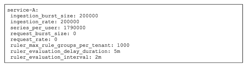
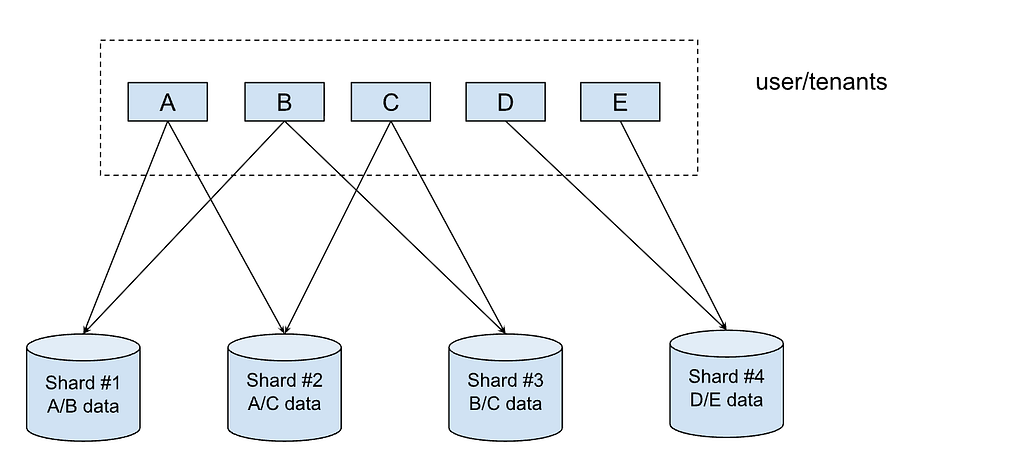
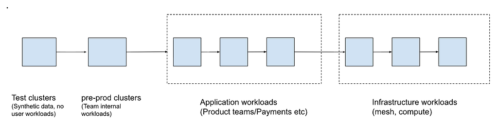




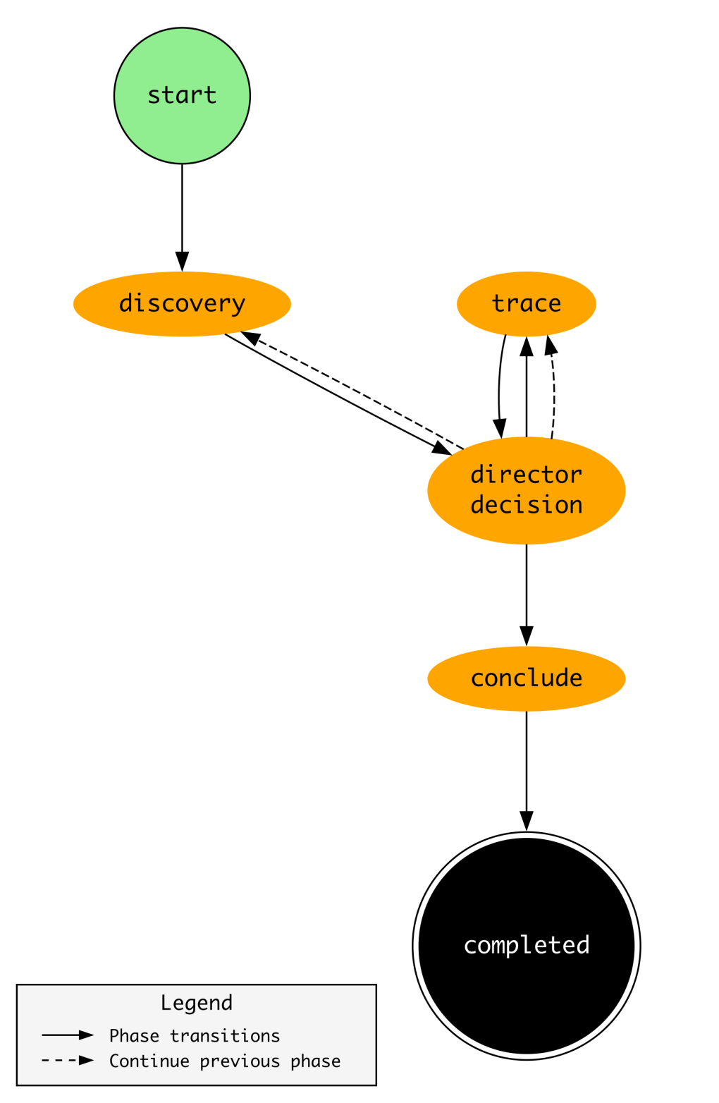
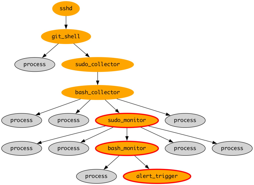


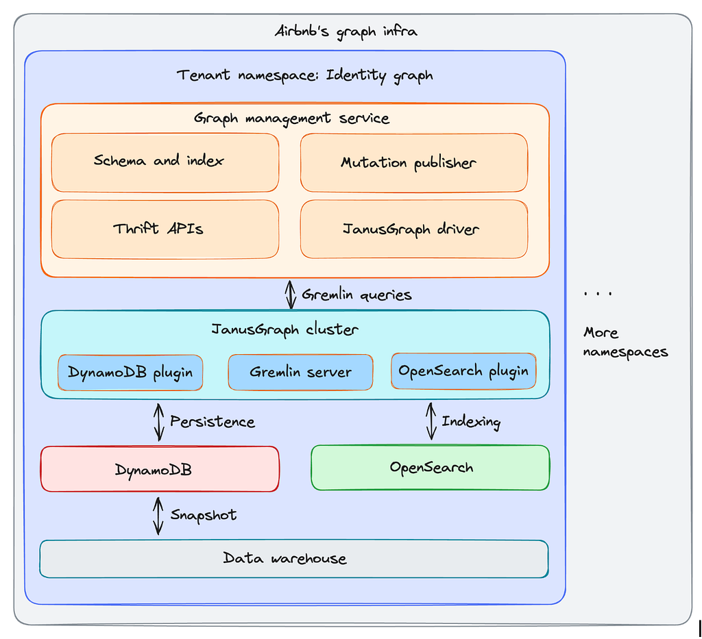
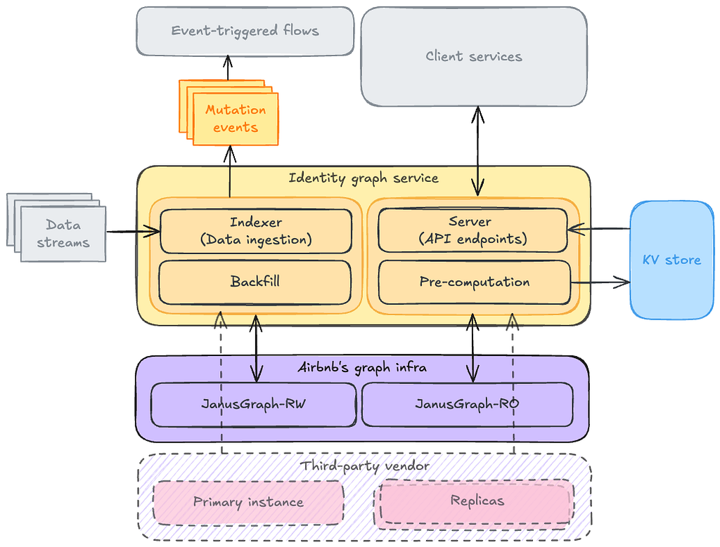
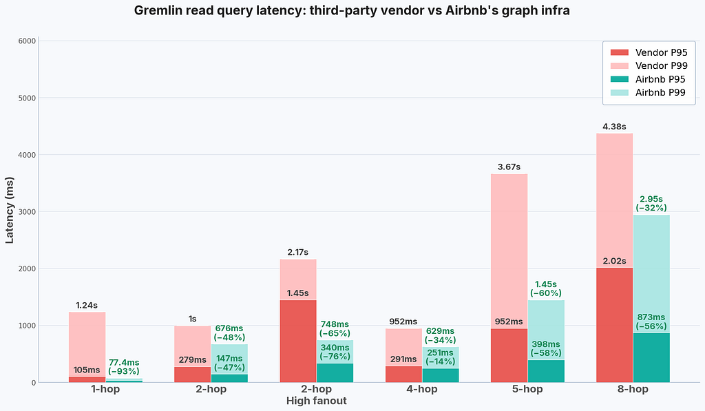
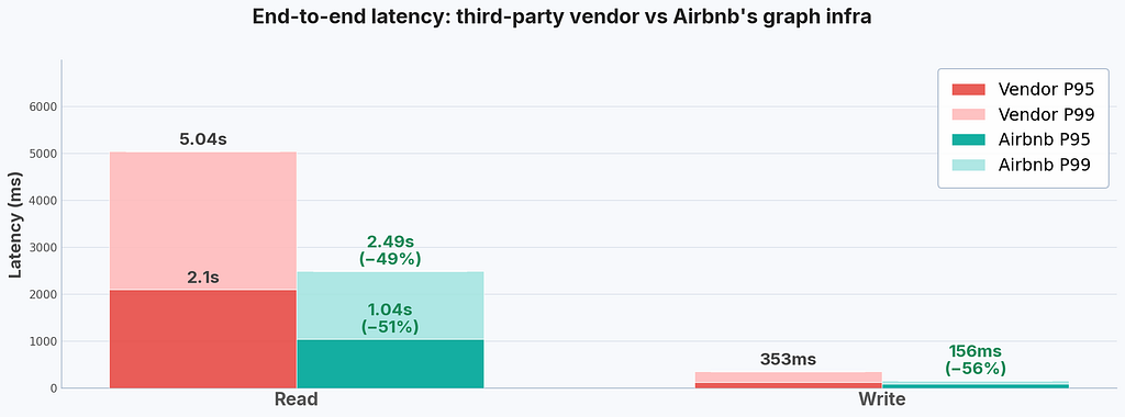
 The capability to handle instant power loss had to be built from the ground up into our DC stack, from mechanical and electrical facilities to server racks, from storage to compute and the core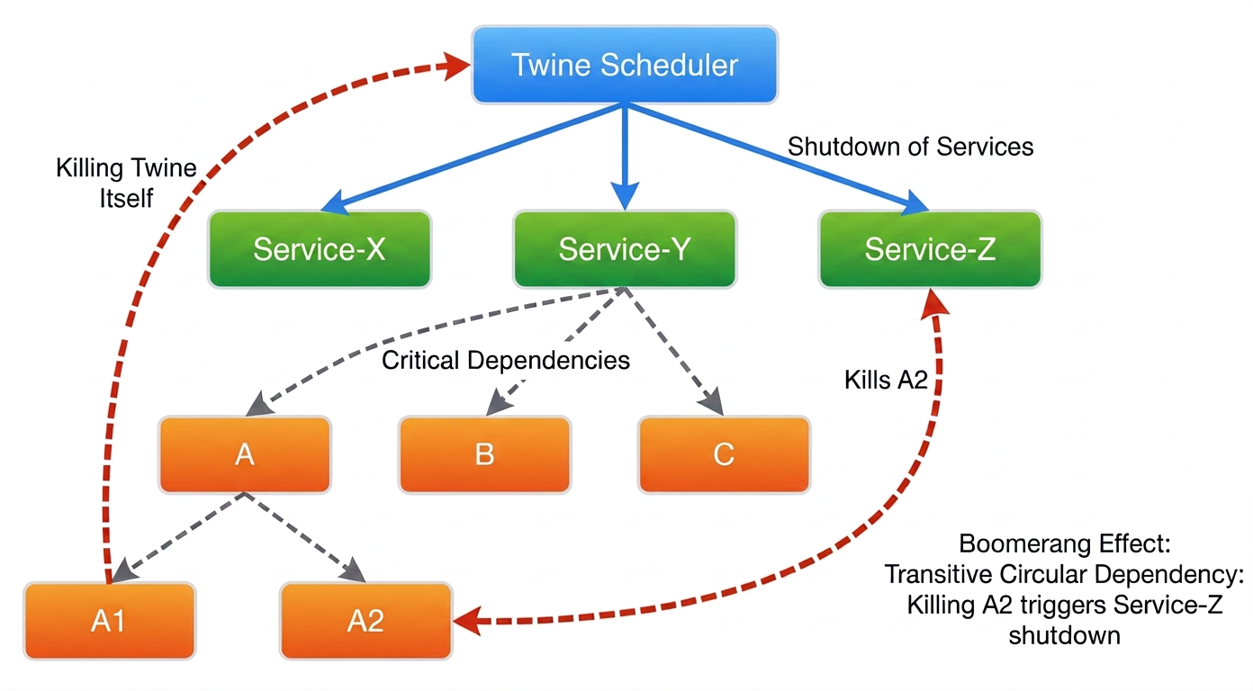


 Four conflicting mental models:
 Hidden coupling between preferences:
 Inconsistent state across clients:
 Power users left behind:



 , guided this project. These weren’t quick bug fixes but rather architecture decisions requiring tight alignment across product, design, frontend, backend, and mobile engineers. We tackled three major technical challenges:




 Users now control noise with confidence.
 Support burden decreased significantly.
 Teams stay informed without the overwhelm.